Received: 11 December 2016 / Revised: 8 April 2017 / Accepted: 18 May 2017
St. Petersburg State University
Saint Petersburg Russia
gaiane-panina@rambler.ru
Abstract
Keywords
Polygonal linkage, Cell complex, CW-complex, Configuration space, Moduli space, Permutohedron, Cyclicpolytope
1.
Preliminaries and Notation

A polygonal $ n$ -linkage is a sequence of positive numbers $ L=(l_1,\dots ,l_n)$. It should be interpreted as a collection of rigid bars of lengths $ l_i$ joined consecutively in a chain by revolving joints. We always assume that the triangle inequality holds, that is, \begin{eqnarray*} \forall j, \ \ \ l_j< \frac{1}{2}\sum_{i=1}^n l_i \end{eqnarray*} which guarantees that the chain of bars can close. A planar configuration of $ L$ is a sequence of points \begin{eqnarray*} P=(p_1,\dots,p_{n}), \ p_i \in \mathbb{R}^2 \end{eqnarray*} with $ l_i=|p_i,p_{i+1}|$, and $ l_n=|p_n,p_{1}|$. We also call $ P$ a polygon .
As follows from the definition, a configuration may have self-intersections and/or self-overlappings.
Definition 1.1.
The moduli space, or the configuration space $ M(L)$ is the set of all configurations of $ L$ modulo orientation preserving isometries of $ \mathbb{R}^2$. Equivalently, we can define $ M(L)$ as \begin{eqnarray*} M(L)=\{(u_1,\ldots,u_n) \in (S^1)^n : \sum_{i=1}^n l_iu_i=0\}/SO(2). \end{eqnarray*}The (second) definition shows that $ M(L)$ does not depend on the ordering of $ \{l_1,\ldots,l_n\}$; however, it does depend on the values of $ l_i$.
Throughout the paper (except for the Sect. 4) we assume that no configuration of $ L$ fits a straight line. This assumption implies that the moduli space $ M(L)$ is a closed $ (n-3)$-dimensional manifold (see [Farber2008]).
The manifold $ M(L)$ is already well studied, see [Farber2008], [Farber and Schütz2007],[Kapovich and Millson1995], and many other papers. Explicit descriptions of $ M(L)$ exist for $ n=4, 5, {\rm and}\, 6$, see [Farber2008],[Kapovich and Millson1995],[Zvonkine1997]. There also exist various results for polygonal linkages in 3D, see [Klyachko1994] for example.
The paper is organized as follows. Section 2 presents an explicit combinatorial description of $ M(L)$ as a regular cell complex $ \mathcal{K}(L)$. In a sense, the starting point of our approach is an elementary version of Gelfand–Goresky–MacPherson–Serganova idea from [Gelfand et al.1987]: they classify the planes (that is, the elements of Grassmanian) by some associated combinatorics. The equivalence classes of the planes form strata which may have complicated topology. In this paper we also classify configurations by their combinatorial types, but here we are lucky with that all equivalence classes are topological balls that patch together in a regular cell complex. The combinatorics of $ \mathcal{K}(L)$ is very much related (but not equal) to the combinatorics of the permutohedron. In Sect. 2 we present a number of examples and give a complete characterization of the possible combinatorics of cells.
In Sect. 3 we study the dual complex $ \mathcal{K}^*$ which comes almost automatically with a geometrical realization in the Euclidean space. The realization is related to cyclopermutohedron [Panina2015], which is a polytope that encodes cyclically ordered partitions of a finite set in the same way as the permutohedron encodes linearly ordered partitions.
Section 4 sketches the main result of [Galashin and Panina2016]: under a proper setting, a "polygonal linkage" can be replaced by a "simple game" (in the game-theoretic sense). A simple game cannot be interpreted as a physical object (like bar-and-joint mechanism) and therefore has no "configurations". However, it is possible to associate with it a cell complex which is proven to be a combinatorial manifold.
Finally, for the sake of completeness, we discuss in Sect. 4 the cell complex for the case when the manifold $ M(L)$ is singular.
The complex $ \mathcal{K}(L)$ already appeared in [Kapovich and Millson1995] in a slight disguise, where it was mentioned as a "tiling of $ M(L)$". Moreover, based on the Deligne-Mostow map, Kapovich and Millson deduced that $ \mathcal{K}(L)$ can be realized as a piecewise linear manifold in the hyperbolic space.
We start with necessary preliminaries. Convex configurations A configuration $ P$ is convex if (1) it is a convex (piecewise linear) curve, (2) no two consecutive edges are collinear, and (3) the orientation induced by the numbering goes counterclockwise.
The set of all convex configurations we denote by $ M_{conv}(L)$. The set $ \overline{M}_{conv}(L)$ is the closure of $ M_{conv}(L)$ in $ M(L)$.
Lemma 1.2.
(M. Kapovich, Personal communications 2013)- (1) The set $ M_{conv}(L)$ is an open subset of $ M(L)$ homeomorphic to the open $ (n-3)$-dimensional ball.
- (2) The closure $ \overline{M}_{conv}(L)$ is homeomorphic to the closed $ (n-3)$-dimensional ball.
- (3) The interior of $ \overline{M}_{conv}(L)$ coincides with $ M_{conv}(L)$.
Proof.
Following paper [Kapovich and Millson1995], consider configurations of $ n$ (not necessarily all distinct) points $ p_i$ in the real projective line $ \mathbb{R}P^1$, which we identify with $ S^1$. Each point $ p_i$ is assigned the weight $ l_i$. The configuration of (weighted) points is called stable if sum of the weights of coiciding points is less than half the weight of all points.The group $ PSL(2,\mathbb{R})$ naturally acts on the space of configurations. A remarkable fact is that the quotient space of stable configurations is exactly the space $ M(L)$. More detailed, take a stable configuration $ \{p_i\}$. We interpret the points $ p_i$ as unit vectors in $ \mathbb{R}^2$. In the orbit of the configuration there exists a unique point (up to rotation of $ S^1$) such that the weighted sum $ \sum l_ip_i$ is zero. Thus each orbit gives a configuration of the linkage $ L$.
A configuration of points yields a convex polygon whenever the numbering $ (1,\ldots,n)$ goes counterclockwise. Therefore $ M_{conv}(L)$ is identified with the set of $ n$-tuples of counterclockwise-oriented distinct points $ x_i$ in $ S^1=\mathbb{R}P^1$ modulo $ PSL(2,\mathbb{R})$. We can omit the action of the group by assuming that the first three points are $ 0,\ 1 $, and $ \infty$. The rest of the points are then given by linear inequalities \begin{eqnarray*} 1< x_4< x_5 < \cdots < x_n < \infty , \end{eqnarray*} which implies the statement (1). The statements (2) and (3) are now straightforward. ⬜
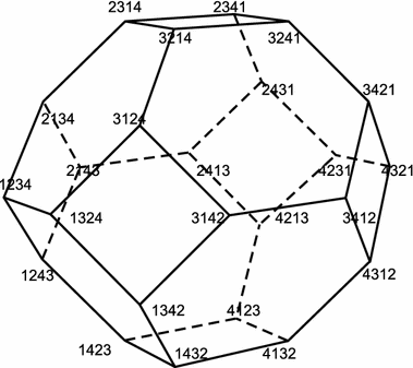
Polytopes We shall use the combinatorial structure of the following polytopes:The permutohedron $ \Pi_n$ (see [Ziegler1995]) is defined as the convex hull of all points in $ \mathbb{R}^n$ that are obtained by permuting the coordinates of the point $ (1,2,\ldots,n)$. It has the following properties:
- (1) $ \Pi_n$ is an $ (n-1)$-dimensional polytope.
- (2) The $ k$-dimensional faces of $ \Pi_n$ are labeled by ordered partitions of the set $ \{1,2,\ldots,n\}$ into $ (n-k)$ non-empty parts. In particular, the vertices are labeled by the elements of the symmetry group $ S_n$. The label of a vertex is obtained by inverting the permutation of the coordinates of the vertex.
- (3) A face $ F'$ of $ \Pi_n$ is contained in a face $ F$ iff the label of $ F'$ is finer than the label of $ F$. Here by a refinement of an ordered partition $ \lambda$ we mean an ordered refinement $ \lambda'$ whose ordering is inherited from $ \lambda$. For instance, $ \{1,3\}\{2,4\}\{5\}$ refines $ \{1,3\}\{2,4,5\}$ and does not refine $ \{2,4,5\}\{1,3\}$.
- (4) A face of $ \Pi_n$ is the Cartesian product of permutohedra of smaller dimensions.
- (5) The permutohedron is a zonotope , that is, the Minkowski sum of line segments.
- (6) The permutohedra $ \Pi_1$, $ \Pi_2$, and $ \Pi_3$ are a one-point polytope, a segment, and a regular hexagon, respectively. The permutohedron $ \Pi_4$ (with its vertices labeled) is depicted in Fig. 1.
The cyclic polytope $ C(d,n)$ is the convex hull of $ n$ distinct points $ x_1,\ldots,x_n$ on the moment curve in $ \mathbb{R}^d$, see [Ziegler1995]. Its combinatorics is completely defined by the following property ( Gale evenness condition ): a $ d$-subset $ F \subset \{x_1,\ldots,x_n\}$ forms a facet of $ C(d,n)$ iff any two elements of $ \{x_1,\ldots,x_n\} {\setminus} F$ are separated by an even number of elements from $ F$ in the sequence $ x_1,\ldots,x_n$.
2. The Complex $ \mathcal{K}(L)$
Assume first that a configuration $ P=(p_1,\ldots,p_n)\in M(L)$ has no parallel edges, that is, no edgevectors $ \overrightarrow{p_ip}_{i+1}$ and $ \overrightarrow{p_jp}_{j+1}$ are parallel and codirected.
Then there exists a unique convex polygon $ \overline{P}$ such that
- (1) The edges of $ P$ are in one-to-one correspondence with the edges of $ \overline{P}$. The bijection preserves the directions of the vectors.
- (2) The orientations of the edges of $ \overline{P}$ give the counterclockwise orientation of $ \overline{P}$.
In other words, the edges of $ \overline{P}$ are the edges of $ P$ coming in the order of their slopes (see Fig. 2). Obviously, $ \overline{P} \in M_{conv}(\lambda L)$ for some permutation $ \lambda \in S_n$. The permutation is defined up to the action of the group generated by the cyclic permutation $ (2,3,4,\ldots,n,1)$. The orbit of a permutation under the action of the group is a cyclic ordering on the set $ [n]$. Summarizing the above, our construction assigns to $ P$ the label $ \lambda(P)$ which is a cyclic ordering on the set $ [n]$. Equivalently, expecting further discussion on polygons with parallel edges, we state that a label of a configuration without parallel edges is a cyclically ordered partition of the set $ [n]=\{1,2,\ldots,n\}$ into $ n$ non-empty parts.
Lemma 2.1.
Given a cyclically ordered partition $ \lambda$ of the set $ [n]$ into $ n$ non-empty parts, the subset of $ M(L)$ of all polygons labeled by $ \lambda$ is an open $ (n-3)$-ball.Proof.
The rearranging construction maps the set of polygons labeled by $ \lambda$ bijectively to $ M_{conv}(\lambda L)$, which is a ball by Lemma 1.2. ⬜Definition 2.2.
Farber and Schütz ([Farber and Schütz2007]) A set $ I\subset [n]=\{1,2,\ldots,n\}$ is called short , if \begin{eqnarray*} \sum_{I}^{}l_i < \frac{1}{2} \sum_{i=1}^{n}l_i. \end{eqnarray*}Definition 2.3.
A partition of the set $ [n]$ is called admissible if all the parts are short.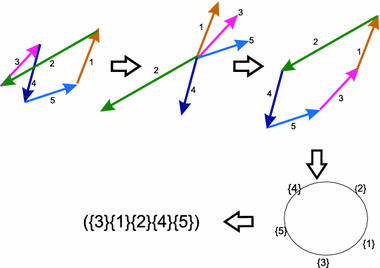
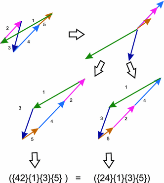
Assume now that a configuration $ P\in M(L)$ has parallel edges. A permutation which makes $ P$ convex is not unique. Indeed, one can choose any ordering on the set of parallel edges. So in cooking the label, our construction puts the indices of parallel edges in one set.
The label $ \lambda(P)$ assigned to $ P$ is a cyclically ordered partition of the set $ [n]$, see Fig. 3 for an example.
Lemma 2.4.
Given a cyclically ordered partition $ \lambda$ of the set $ [n]$ into $ k$ non-empty sets, the subset of $ M(L)$ of all polygons labeled by $ \lambda$ is either an open $ (k-3)$-ball (if $ \lambda$ is an admissible partition), or an empty set (if $ \lambda$ is non-admissible).Proof.
We apply Lemma 2.1 to the $ k$-bar linkage with frozen together edges. Namely, we replace each collection of edges with equal slopes by a single edge. ⬜ A remark on notation We write a cyclically ordered partition as a (linearly ordered) string of sets where the set containing the entry "$ n$" stands on the last position.We stress once again that the order of the sets matters, whereas there is no ordering inside a set. For example, \begin{eqnarray*} (\{1\} \{3 \} \{4, 2, 5,6\})\neq(\{3 \}\{1\} \{4, 2, 5,6\})= ( \{3 \}\{1\}\{ 2,4, 5,6\}). \end{eqnarray*}
Definition 2.5.
Two points from $ M(L)$ (that is, two configurations) are equivalent if they have one and the same label. Equivalence classes of $ M(L)$ we call the open cells . The closure of an open cell in $ M(L)$ is called a closed cell . By above lemmata, all cells are homeomorphic to balls.For a cell $ C$, either closed or open, its label $ \lambda (C)$ is defined as the label of any interior point of the cell.
Before we formulate the main theorem, remind that a CW-complex can be constructed inductively by defining its skeleta. Once the $ (k - 1)$-skeleton is constructed, we attach a collection of closed $ k$-balls $ C_i$ by some continuous mappings $ \varphi_i$ from their boundaries $ \partial C_i$ to the $ (k-1)$-skeleton. For a regular complex, each of the mappings $ \varphi_i$ is injective, and $ \varphi_i$ maps $ \partial C_i$ to a subcomplex of the $ (k-1)$-skeleton, see [Hatcher2002]. Regularity of a complex implies that a complex is uniquely defined by the poset of its cells. Regularity also guarantees the existence of well-defined barycentric subdivision and (for PL manifolds) a well-defined dual complex.
Theorem 2.6.
The above described collection of cells yields a structure of a regular CW-complex $ \mathcal{K}(L)$ on the moduli space $ M(L)$. Its complete combinatorial description reads as follows:- (1) $ k$-cells of the complex $ \mathcal{K}(L)$ are labeled by cyclically ordered admissible partitions of the set $ [n]$ into $ (k+3)$ non-empty parts.
- (2) A closed cell $ C$ belongs to the boundary of some other closed cell $ C'$ iff the partition $ \lambda(C')$ is finer than $ \lambda(C)$.
Proof.
The open cells are balls by Lemmata 2.1 and 2.4. The regularity of the complex follows from Lemma 1.2, (3). ⬜For the complex $ \mathcal{K}(L)$ we immediately have:
Proposition 2.7.
- (1) The facets of the complex (that is, the cells of maximal dimension $ n-3$) are labeled by cyclic orderings on the set $ [n]$.
- (2) The vertices of the complex are labeled by cyclically ordered admissible partitions of the set $ [n]$ into three non-empty parts. In other words, they correspond to all possible (oriented) triangles composed of segments of lengths $ l_1,\ldots,l_n$.
- (3) The vertex figure of any vertex $ v$ of the complex $ \mathcal{K}(L)$ is combinatorially dual to the Cartesian product of three permutohedra. More precisely, the label $ \lambda(v)$ consists of three parts. If the three parts have $ k$, $ l$, and $ m$ elements, respectively, then the vertex figure of $ v$ is combinatorially dual to $ \Pi_k\times \Pi_l \times \Pi_m$.
- (4) The face figure of any $ k$-dimensional face is combinatorially dual to the Cartesian product of $ (k+3)$ permutohedra (some of these permutohedra can be $ \Pi_1$, and thus degenerate to a point).
Proof.
The proof follows directly from the above construction. ⬜Example 2.8.
Let $ n=4; \ \ l_1=l_2=l_3=1,\ l_4=1/2.$ The moduli space $ M(L)$ is known to be a disjoint union of two circles, see [Farber2008]. The cell complex $ \mathcal{K}(L)$ is depicted in Fig. 4.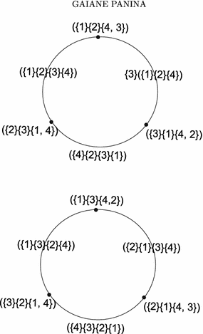
Example 2.9.
Assume that \begin{eqnarray*} \forall i \ \ l_n+l_i> \sum_{ n\neq j\neq i} l_j. \end{eqnarray*} In this case the moduli space $ M(L)$ is an $ (n-3)$-sphere, see [Farber2008], and the complex $ \mathcal{K}(L)$ is dual to the boundary complex of the permutohedron $ \Pi_{n-1}$.Proof.
Indeed, each admissible partition is of the type \begin{eqnarray*} (*, \{n\}), \end{eqnarray*} where "$ *$" is any linearly ordered partition of $ [n-1]$ in at least two parts. This means that the facets of $ \mathcal{K}(L)$ are in a natural bijection with the vertices of $ \Pi_{n-1}$. It remains to observe that the patching rules for $ \mathcal{K}(L)$ are exactly dual to those of the permutohedron. ⬜In a regular complex, the boundary of each cell is a combinatorial sphere, so it makes sense to speak of combinatorics of a cell. Let us look what types of combinatorics do we encounter in complexes $ \mathcal{K}(L)$ for different linkages $ L$.
Example 2.10.
Let $ n=5$, $ L=(1,1,1,1,1)$. Then $ \mathcal{K}(L)$ is a surface of genus four patched of 24 pentagons. Each vertex has $ 4$ incident edges. The complex is flag-transitive , which means that any combinatorial equivalence of any two pentagons extends to an automorphism of the entire complex.Example 2.11.
Let $ n=2k+1$, $ L=(1,1,\ldots,1)$. Then $ \mathcal{K}(L)$ is patched of $ (2k)!$ copies of duals to the cyclic polytope $ C(n-3,n)$.However, unlike the previous example, the complex is not completely transitive, just facet-transitive : for every two facets there exists an automorphism of $ \mathcal{K}(L)$ mapping one facet to the other.
Proof.
Fix a facet $ C$ of $ \mathcal{K}(L)$. Without loss of generity we may assume that its label is $ (\{1\}\{2\}\{3\}\{4\}\ldots\{n\})$. Consider the following "starlike" bijection $ \varphi$ which maps the vertices $ x_1,\ldots,x_n$ of the cyclic polytope $ C(n-3,n)$ to facets of the cell $ C$: \begin{eqnarray*} &&\varphi(x_{2i+1})=(\{1\}\{2\}\{i+1,i+2\}\{3\}\{4\}\ldots\{n\}),\\ &&\varphi(x_{2i})=(\{1\}\{2\}\{k+i-1,k+i\}\{3\}\{4\}\ldots\{n\}). \end{eqnarray*} Informally, the defining rule of $ \varphi$ is the way of drawing a polygonal star (say, a pentagram). It is easy to check that $ \varphi$ yields a combinatorial duality. ⬜Proposition 2.12.
- (1) Faces of $ \mathcal{K}(L)$ are combinatorially equivalent to convex polytopes Let $ C$ be a closed cell of $ \mathcal{K}(L)$ for some polygonal linkage $ L$. The boundary complex of $ C$ is combinatorially equivalent to a simple $ k$-polytope with at most $ k+3$ facets. Moreover, there exists some even $ D\in \mathbb{N}$ such that the boundary complex of $ C$ is combinatorially equivalent to a face of the dual to the cyclic polytope $ C(D,D+3)$.
- (2) Universality property Conversely, any simple $ k$-dimensional polytope $ K$ with at most $ k+3$ facets arises in this way. That is, there exist a number $ n$, an $ n$-linkage $ L$, and a cell $ C$ of the complex $ \mathcal{K}(L)$ such that the boundary complex of $ C$ is combinatorially equivalent to $ K$.
Proof.
- (1) We may assume that all $ l_i$ are integers, and that their sum $ D+3=\sum l_i$ is odd. Indeed, neither a small perturbation nor a scaling changes the combinatorics of the complex. The space $ M(L)$ embeds in a natural way in the moduli space of the equilateral polygon with $ D+3$ edges $ M(\underbrace{1,1,\ldots,1}_{D+3}).$ The embedding maps a polygon with edgelengths $ l_1,\ldots,l_n$ to the equilateral polygon which represents the same curve, that is, with first $ l_1$ edges parallel, next $ l_2$ edges parallel, etc. The embedding respects the structure of cell complexes, and therefore, realizes $ \mathcal{K}(L)$ as a subcomplex of the complex $ \mathcal{K}(\underbrace{1,1,\ldots,1}_{D+3})$, whose facets are combinatorial cyclic polytopes (see Example 2.11).
- (2) Assume that a simple $ k$-dimensional polytope $ K$ has $ k+3$ facets. Then the dual polytope $ K^*$ has $ k+3$ vertices. We shall prove that every simplicial $ k$-polytope with at most $ k+3$ vertices is a face figure of the cyclic polytope $ C(D,D+3)$ for some even $ D$. The Gale diagram of $ K^*$ (see [Ziegler1995]) is a one-dimensional configuration of distinct black and white points. Remind that the Gale diagram of $ C(D,D+3)$ is the alternating configuration of distinct black and white points in the straight line. Being translated to the Gale diagram's language, the statement we need reads as "any configuration of distinct black and white points in the straight line can be completed to an alternating configuration of distinct black and white points", which is obvious. If $ K$ has less than $ k+3$ facets, the proof is even simpler.
3.
The Dual Complex $ \mathcal{K}^*(L)$: Surgery on the Permutohedron
Theorem 3.1.
The dual cell complex $ \mathcal{K}^*(L)$ carries a natural structure of a polyhedron.Proof.
The cells of the dual complex $ \mathcal{K}^*$ are the duals to the face figures of $ \mathcal{K}(L)$. By Theorem 2.6, the latter are combinatorially equivalent to Cartesian products of permutohedra. To realize $ \mathcal{K}^*$ as a polyhedron, for each facet of $ \mathcal{K}^*$ we take the Cartesian product of three standard permutohedra. Their faces that are identified via isometries. ⬜We describe below a realization of $ \mathcal{K}^*$ in the Euclidean space $ \mathbb{R}^{n-2}$. For this, we need a preliminary construction which is the subject of paper [Panina2015]. The construction involves the theory of virtual polytopes developed originally in [Pukhlikov and Khovanskii1993], and some related technique. For the very first orientation we recommend the reader just to trust that there exists a well-defined Minkowski subtraction of convex polytopes, and that Minkowski differences have a well-defined facial structure. For more details, we refer to the above mentioned paper. Cyclopermutohedron For a fixed number $ n\geq3$, we define the following regular cell complex $ {CP}_{n}$ by listing all the closed cells together with the incidence relations.
- For $ k=0,\ldots,n-3$, the $ k$-dimensional cells ($ k$-cells, for short) of the complex $ {CP}_{n}$ are labeled by (all possible) cyclically ordered partitions of the set $ [n]$ into $ (n-k)$ non-empty parts.
- A (closed) cell $ F$ contains a cell $ F'$ whenever the label of $ F'$ refines the label of $ F$.
The complex $ {CP}_{n}$ cannot be represented by a convex polytope, since it is not a combinatorial sphere (not even a combinatorial manifold). However, it can be represented by some virtual polytope which we call cyclopermutohedron $ \mathcal{CP}_{n}$.
Here is the construction of cyclopermutohedron:
Assuming that $ \{e_i\}$ are standard basic vectors in $ \mathbb{R}^{n-1}$, define the points \begin{eqnarray*} \begin{array}{ccccccccc} R_i=\sum_{j=1}^{n-1} (e_j-e_i)=(-1, & \ldots & -1, & n-2, & -1, & \ldots & -1, & -1, &-1, )\in \mathbb{R}^{n-1},\\ & & & \ i & & & & & \end{array} \end{eqnarray*} and the following two families of line segments: \begin{eqnarray*} q_{ij}=\left[e_i,e_j\right], \ \ \ i< j \end{eqnarray*} and \begin{eqnarray*} r_i=\left[0,R_{i} \right]. \end{eqnarray*} We also need the point $ S=\left(1,1,\ldots,1\right)\in \mathbb{R}^{n-1}$.
Definition 3.2.
The cyclopermutohedron is a virtual polytope defined as the weighted Minkowski sum of line segments: \begin{eqnarray*} \mathcal{CP}_{n}:= \sum_{i< j} q_{ij} + S- \sum_{i=1}^{n-1} r_i. \end{eqnarray*}Theorem 3.3.
[Panina2015] The poset of (proper) faces of $ \mathcal{CP}_{n}$ is combinatorially isomorphic to the complex $ CP_{n}$.Remark.
The sum $ S+ \sum_{i< j} q_{ij}$ equals the standard permutohedron.In an oversimplified way, the cyclopermutohedron $ \mathcal{CP}_{n}$ can be visualized as the permutohedron $ \Pi_{n-1}$ "with diagonals". This means that all the proper faces of $ \Pi_{n-1}$ are also faces of $ \mathcal{CP}_{n}$. However, $ \mathcal{CP}_{n}$ has some extra faces in comparison with $ \Pi_{n-1}$.
For any $ n$-linkage $ L$, the complex $ \mathcal{K}^*(L)$ automatically embeds in $ {CP}_{n}$, and therefore embeds in the face complex of $ \mathcal{CP}_{n}$. The embedding goes as follows. Take the permutohedron $ \Pi_{n-1}\subset \mathbb{R}^{n-1}$, assuming (as usual) that the faces of $ \Pi_{n-1}$ are labeled by ordered partitions on the set $ [n-1]$. In particular, the vertices of $ \Pi_{n-1}$ are labeled by permutations of the set $ [n-1]$. We introduce the following bijection between the vertex sets \begin{eqnarray*} \psi: Vert(\mathcal{K}^*)\rightarrow Vert(\Pi_{n-1}). \end{eqnarray*} Given a vertex of $ \mathcal{K}^*$ whose label $ \lambda$ is a cyclically ordered set $ [n]$, the mapping $ \psi$ sends it to the vertex of $ \Pi_{n-1}$ by cutting $ \lambda$ at the position of "$ \{n\}$" and omitting "$ \{n\}$" from the label.
Thus, the vertices of $ \mathcal{K}^*$ are geometrically realized by vertices of the permutohedron. Next, we realize the cells of the complex: take a cell $ C$ and patch the face of the cyclopermutohedron which corresponds to $ C$ by Theorem 3.3.
This construction can be reformulated as the following surgery algorithm:
- (1) Start with the complex $ \mathcal{K}^*(L)$ and the boundary complex of the permutohedron $ \Pi_{n-1}$. Realize the vertices of $ \mathcal{K}^*$ as the vertices of $ \Pi_{n-1}$ via the above described mapping $ \psi$.
- (2) For every face $ F$ of $ \Pi_{n-1}$ do the following. The face is labeled by some $ \lambda$, which is a linearly ordered partition of $ \{1,\ldots,n-1\}$. If the partition is admissible (that is, all the parts are short), keep the face $ F$ and assign to it the label $ (\lambda, \{n\})$. If the partition is not admissible, remove the face $ F$ from the complex. This step gives a realization of all the cells of $ \mathcal{K}^*$ whose label contains the one-element set $ \{n\}$.
- (3) Take all the cells $ C$ of $ \mathcal{K}^*$ such that the part of $ \lambda(C)$ containing $ n$ has more than one element. Patch in the corresponding face of the cyclopermutohedron, which up to a translation equals \begin{eqnarray*} \sum q_{ij} - \sum r_i, \end{eqnarray*} where the first (Minkowski) sum extends over all $ i< j< n$ such that $ i$ and $ j$ belong to one and the same part of the partition $ \lambda(C)$, and the second sum extends over all $ i< n$ such that $ i$ and $ n$ belong to one and the same part of the partition $ \lambda(C)$. This is a virtual polytope with the vertex set $ \psi (Vert(C))$.
Example 3.4.
Let $ L$ be as in Example 2.9. The above described surgery leaves the permutohedron as it is. That is, all the faces of $ \ \Pi_{n-1}$ survive on the second step of the surgery algorithm, and nothing is added on the third step.Important is that the "long" edge is the last one. Otherwise we would get another surgery, but, of course, an isomorphic combinatorics.
Example 3.5.
Let $ n=5$; $ l_1=1,2;\ l_2=1;\ l_3=1;\ l_4=0,8;\ l_5=2,2$. The surgery algorithm starts with the permutohedron $ \Pi_4$ (see Fig. 5). The two shadowed faces are labeled by $ (\{123\}\{4\})$ and $ (\{4\}\{123\})$. Since the partitions $ (\{123\}\{4\}\{5\})$ and $ (\{4\}\{123\}\{5\})$ are non-admissible, according to the algorithm, the faces are removed. All other faces of the permutohedron survive the surgery. Step 3 gives six new "diagonal" rectangular faces. They correspond to the cells labeled by $ (\{1\}\{2\}\{3\}\{45\})$, $ (\{1\}\{3\}\{2\}\{45\})$, $ (\{2\}\{1\}\{3\}\{45\})$, $ (\{2\}\{3\}\{1\}\{45\})$, $ (\{3\}\{1\}\{2\}\{45\})$, and $ (\{3\}\{2\}\{1\}\{45\})$.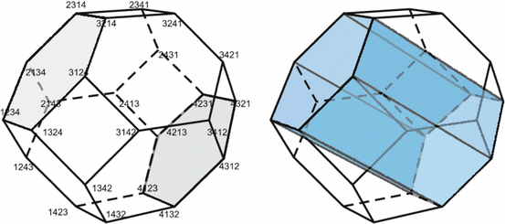
Example 3.6.
Let $ n=5$, $ L=(3,\ 1,\ 1,\ 4,\ 4)$. Figure 6 presents the permutohedron, the labels of the vertices, and the coordinates of the vertices (in bold). We also depict the hexagonal face labeled by $ (\{1\}\{4\}\{235\})$. It is the Minkowski sum of two negatively weighted and one positively weighted segments.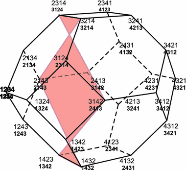
For more examples of the surgery see [Gorodetskaya2017], where Gorodetskaya presented the surgery for all types of five-linkages.
4. Concluding Remarks
The construction of $ \mathcal{K}$ and $ \mathcal{K}^*$ suggests some further natural discussions sketched briefly in this section. Quasilinkages, Simple Games, Alexander Self-Dual Complexes, and Associated Manifolds An elementary observation is that the complex $ \mathcal{K}(L)$ depends only on the collection of admissible partitions. In turn, these are defined by the collection of short sets. This suggests the following generalization, which is described in details in [Galashin and Panina2016], and which we sketch very briefly now.
Definition 4.1.
A family $ \mathcal{F}$ of subsets of $ [n]$ is called a quasilinkage , if it satisfies the following properties:- (1) $ \mathcal{F}$ contains all singletons: for any $ i \in [n]$, $ \{i\} \in \mathcal{F}$.
- (2) Monotonicity: if $ S\in \mathcal{F}$, and $ T\subset S$ then $ T\in \mathcal{F}$.
- (3) Strong complementarity: if $ S\in \mathcal{F}$ then $ ([n]{\setminus} S)\notin \mathcal{F}$ , and, conversely, if $ S\notin \mathcal{F}$, then $ ([n]{\setminus} S)\in \mathcal{F}$.
The proposed notion exists in the literature; yet in completely different frameworks. It appeared as "simple game with constant sum" in game theory, as "strongly complementary simplicial complex", and as "Alexander self-dual simplicial complex".
Being motivated by polygonal linkages, we call any $ S\in \mathcal{F}$ a short set , and any $ S\notin \mathcal{F}$ a long set .
Each polygonal linkage $ L$ yields a collection of short sets, and therefore, is a quasilinkage. The converse is not true: there exist many quasilinkages that cannot be represented by length assignments.
We associate with a quasilinkage $ \mathcal{F}$ a cell complex $ \mathcal{K}(\mathcal{F})$ by applying the rules from Theorem 2.6. In [Galashin and Panina2016] it is proven that the complex is a (combinatorial) manifold of dimension $ (n-3)$ which is locally isomorphic to $ \mathcal{K}(L)$ for some linkage $ L$ (however, $ L$ depends on the location, and there may be no linkage associated to the entire complex). Cell Decomposition for Singular Configuration Spaces A similar cell complex exists also for singular configuration spaces, that is, for the case when $ L$ has configurations that fit in a straight line.
Definition 4.2.
For a singular case, a partition of $ L=(l_1,\dots ,l_n)$ is called admissible if one of the two conditions holds:- (1) The number of the parts is greater than $ 2$, and the total length of any part is strictly greater than the total length of the rest.
- (2) The number of parts equals $ 2$, and the lengths of the parts are equal.
The combinatorics of the complex $ \mathcal{K}(L)$ is literally the same as in Theorem 2.6 except for the following items:
- (1) Non-singular vertices are labeled by admissible partitions with exactly three parts.
- (2) Singular vertices are labeled by admissible partitions with exactly two parts.
- (3) Assume that a singular vertex $ v$ of $ \mathcal{K}(L)$ corresponds to an ordered partition of $ \{1,2,\ldots,n\}$ into two non-empty parts, say, with $ k$ and $ l$ elements. Then the vertex figure of $ v$ is combinatorially equivalent to the cone over $ (\partial \Pi_k\times \partial \Pi_l)^* $.
Acknowledgements.
I am grateful to Nikolai Mnev for inspiring conversations. I am also indebted to Misha Kapovich for delivering me the proof of Lemma 1.2.References
[Farber2008] Farber, M.: Invitation to topological robotics. Zuerich lectures in advanced mathematics. European Mathematical Society (EMS), Zuerich (2008)
[Farber and Schütz2007] Farber, M., Schütz, D.: Homology of planar polygon spaces. Geom. Dedicata 125 , 75-92 (2007)
[Hatcher2002] Hatcher, A.: Algebraic Topology. Cambridge University Press, Cambridge (2002)
[Gelfand et al.1987] Gelfand, I., Goresky, M., MacPherson, R., Serganova, V.: Combinatorial geometries, grassmannians, and the moment map. Adv. Math 63 , 301-316 (1987)
[Gorodetskaya2017] Gorodetskaya, I.: Moduli spaces of planar pentagonal linkages: combinatorial description. arXiv:1305.6756
[Kapovich and Millson1995] Kapovich, M., Millson, J.: On the moduli space of polygons in the Euclidean plane. J. Diff. Geom. 42 , 430-464 (1995)
[Klyachko1994] Klyachko, A.: Spatial polygons and stable configurations of points in the projective line. In: Tikhomirov A., et al. (eds.) Algebraic Geometry and Its Applications, Proceedings of the 8th Algebraic Geometry Conference, Yaroslavl', Russia, August 10-14, 1992. Braunschweig: Vieweg. Aspects Math. E 25, 67-84 (1994)
[Pukhlikov and Khovanskii1993] Pukhlikov, A., Khovanskii, A.: Finitely additive measures of virtual polyhedra. St. Petersburg Math. J. 4 (2), 337-356 (1993)
[Panina2015] Panina, G.: Cyclopermutohedron. Trudy Mian 288 , 149-162 (2015)
[Ziegler1995] Ziegler, G.: Lectures on Polytopes. Graduate Texts in Mathematics, vol. 152. Springer, New York (1995)
[Zvonkine1997] Zvonkine, D.: Configuration spaces of hinge constructions. Russ. J. Math. Phys. 5 (2), 247-266 (1997)
- 99
- × Galashin, P., Panina, G.: Manifolds associated to simple games. J. Knot Theory Ramif. 25 (12), (2016). doi:
- × Farber, M.: Invitation to topological robotics. Zuerich lectures in advanced mathematics. European Mathematical Society (EMS), Zuerich (2008)
- × Farber, M., Schütz, D.: Homology of planar polygon spaces. Geom. Dedicata 125 , 75-92 (2007)
- × Hatcher, A.: Algebraic Topology. Cambridge University Press, Cambridge (2002)
- × Gelfand, I., Goresky, M., MacPherson, R., Serganova, V.: Combinatorial geometries, grassmannians, and the moment map. Adv. Math 63 , 301-316 (1987)
- × Gorodetskaya, I.: Moduli spaces of planar pentagonal linkages: combinatorial description. arXiv:1305.6756
- × Kapovich, M., Millson, J.: On the moduli space of polygons in the Euclidean plane. J. Diff. Geom. 42 , 430-464 (1995)
- × Klyachko, A.: Spatial polygons and stable configurations of points in the projective line. In: Tikhomirov A., et al. (eds.) Algebraic Geometry and Its Applications, Proceedings of the 8th Algebraic Geometry Conference, Yaroslavl', Russia, August 10-14, 1992. Braunschweig: Vieweg. Aspects Math. E 25, 67-84 (1994)
- × Pukhlikov, A., Khovanskii, A.: Finitely additive measures of virtual polyhedra. St. Petersburg Math. J. 4 (2), 337-356 (1993)
- × Panina, G.: Cyclopermutohedron. Trudy Mian 288 , 149-162 (2015)
- × Ziegler, G.: Lectures on Polytopes. Graduate Texts in Mathematics, vol. 152. Springer, New York (1995)
- × Zvonkine, D.: Configuration spaces of hinge constructions. Russ. J. Math. Phys. 5 (2), 247-266 (1997)