Received: 23 March 2017 / Revised: 10 June 2017 / Accepted: 2 August 2017
Sophie Morier-Genoud Sorbonne Universités, UPMC Univ Paris 06, Institut de Mathématiques de Jussieu-Paris Rive Gauche, UMR 7586, CNRS, Univ Paris Diderot, Sorbonne Paris Cité 75005 Paris France sophie.morier-genoud@imj-prg.fr, Valentin Ovsienko CNRS, Laboratoire de Mathématiques U.F.R. Sciences Exactes et Naturelles Moulin de la Housse BP 1039 51687 Reims Cedex 2 France valentin.ovsienko@univ-reims.fr
Abstract
Keywords
Schubert variety, Singularity, Tangent cone, Rank matrix, Essential set
1.
Introduction 
Let $ \F$ be the algebraic variety of all complete flags in $ \Csps^n$. Recall that a complete flag $ F\in\F$ is an increasing sequence of subspaces \begin{equation*} \{0\}=V_0\subset{}V_1\subset{}V_2\subset\cdots\subset{}V_n=\Csps^n, \quad \dim{}V_k=k. \end{equation*} Choosing the standard basis $ \{\e_1,\ldots,\e_n\}$ of $ \Csps^n$, one defines the standard flag, $ F_0\in\F$, for which $ V_k=\Csps^k:=\langle\e_1,\ldots\e_k\rangle$, for all $ 1\leq{}k\leq{}n$. The group $ \GL(n,\Csps)$ of linear transformations of $ \Csps^n$ transitively acts on $ \F$. The Borel subgroup $ B\subset\GL(n,\Csps)$ of upper-triangular matrices is the stabilizer of the standard flag $ F_0$, so $ \F=\GL(n,\Csps)/B$.
Let us recall some well-known facts. The group $ B$ acts naturally on $ \F$ (by left multiplication). The variety $ \F$ is a disjoint union of $ B$-orbits called Schubert cells . Schubert cells are indeed cells of the most classical CW decomposition of $ \F$. Schubert cells are parametrized by elements of the symmetric group $ S_n$. Namely, the group $ S_n$ acts naturally in $ \Csps^n$, and hence in $ \F$, and for every $ w\in S_n$, there exists a unique Schubert cell, which contains the $ w$-image of the standard flag $ F_0$. We denote this cell by $ {\mathcal C}_w$. Its complex dimension is equal to the length of $ w$, i.e., the minimal $ \ell$ in a decomposition \begin{eqnarray*} w=s_{i_1}s_{i_2}\cdots{}s_{i_\ell}, \end{eqnarray*} where $ s_i\in{}S_n$ are the elementary transpositions. The number of Schubert cells of complex dimension $ m$ is the coefficient at $ t^m$ in the polynomial \begin{eqnarray*} \prod_{k=1}^n(1+t+\cdots+t^k). \end{eqnarray*} In particular, there is a unique 0-dimensional cell, which is $ F_0$, and a unique $ \frac{n(n-1)}2$-dimensional cell, which is dense in $ \F$.
The closure $ \X_w$ of a Schubert cell $ {\mathcal C}_w$ is called a Schubert variety . The Schubert variety $ \X_w$ is the union of the Schubert cell $ {\mathcal C}_w$ and all Schubert cells $ {\mathcal C}_{w'}$ corresponding to permutations $ w'$ which precede $ w$ with respect to the natural partial ordering of $ S_n$ (the Bruhat order). In particular, every Schubert variety contains the point $ F_0$.
With a Schubert variety $ \X_w$, we associate two subsets of the tangent space $ T_{F_0}\F$:
- the tangent cone $ \T_w$, which is the set of vectors tangent to $ \X_w$ at $ F_0$;
- the Zariski tangent space $ \mathcal{Z}_w$ which is spanned by $ \T_w$.
Certainly, the Schubert varieties $ \X_w$ and $ \X_{w'}$ coincide only when $ w=w'$; however, the equalities $ {\mathcal Z}_w={\mathcal Z}_{w'}$ or $ \T_w=\T_{w'}$ may occur for $ w\neq w'$ (since the second implies the first, the first occurs "more often" than the second).
For the further discussion, let us introduce the most natural local coordinate system in a (Zariski) neighborhood of $ F_0$ in $ \F$. For a flag $ \{V_k\}$ sufficiently "close" to $ F_0$, there exists a unique "triangular" basis in $ \Csps^n$, \begin{eqnarray*} v_1= \left( \begin{array}{l} 1\\ x_{21}\\ x_{31}\\ \vdots\\ x_{n1} \end{array} \right), \qquad v_2= \left( \begin{array}{l} 0\\ 1\\ x_{32}\\ \vdots\\ x_{n2} \end{array} \right), \quad\dots,\qquad v_n= \left( \begin{array}{l} 0\\ 0\\ \vdots\\ 0\\ 1 \end{array} \right) \end{eqnarray*} such that $ V_k$ is spanned by $ v_1,\dots,v_k$. The numbers $ x_{ij},i> j$, are coordinates of the flag $ \{V_k\}$ (with $ F_0=(0,\dots,0)$); the same numbers may be regarded as coordinates in $ T_{F_0}\F$. (This coordinate system provides a natural identification of $ T_{F_0}\mathcal F$ with the space $ {\mathfrak n}_-$ of strictly lower triangular matrices.) When $ n$ is not too large, we will use the more convenient notations $ x_i=x_{i,i+1},y_i=x_{i,i+2}$, etc.
Zariski tangent spaces $ {\mathcal Z}_w$ were thoroughly studied, see ([Polo1994], [Lakshmibai1995], [Billey and Lakshmibai2000]) and references therein. The following result of Lakshmibai ([Lakshmibai1995]) provides an explicit description of $ {\mathcal Z}_w$. The space $ {\mathcal Z}_w$, viewed as a subspace of $ {\mathfrak n}_-$, is the linear span of the elements $ e_{-\alpha}$ of the Chevalley basis, such that \begin{eqnarray*} \alpha\in R^+,\; s_\alpha\leq w, \end{eqnarray*} where $ R^+$ is the set of positive roots, and $ s_\alpha\in S_n$ is the reflection associated with $ \alpha$, and $ \leq$ is the Bruhat order. The above result, of course, answers the question, under which condition two different Schubert varieties $ \X_w$ and $ \X_{w'}$ have the same Zariski tangent space. On the contrary, the structure of tangent cones $ \T_w$, although it has been an active area of research (see [Billey and Lakshmibai2000], [Brion2005], [Carrell and Kuttler2006], [Eliseev and Panov2013], [Bochkarev et al.2016], [Ignatyev and Shevchenko2015] and references therein), is not well understood, in particular, the problem of their coincidence is mostly open.
Let us consider some examples. If $ n=3$, then $ \dim\F=3$ and the local coordinates are $ x_1,x_2,y$. There are 6 Schubert varieties of dimensions $ 0,1,1,2,2,3$, and the middle four are: \begin{eqnarray*} \X_{213}=\{V_1=\Csps^1\},\quad \X_{213}=\{V_2=\Csps^2\}, \quad \X_{231}=\{V_1\subset\Csps^2\},\quad \X_{312}=\{V_2\supset\Csps^1\}. \end{eqnarray*} In our local coordinates these are $ x_1=y=0, \, x_2=y=0, \, y=0,\, y=x_1x_2$, respectively. We see that, within the domain of our coordinate system, $ \X_{231}$ is the tangent plane (at the origin) to $ \X_{312}$; thus $ \T_{231}=\T_{312}={\mathcal Z}_{231}={\mathcal Z}_{312}$.
The first examples of singular Schubert varieties appear when $ n=4$. There are two of them, cf. ([Lakshmibai and Sandhya1990]): \begin{eqnarray*} \X_{3412}=\{V_1\subset\Csps^3,\, \Csps^1\subset V_3\} \quad\hbox{and}\quad \X_{4231}=\{V_2\cap\Csps^2\neq0\}. \end{eqnarray*} Our local coordinates in the 6-dimensional manifold $ \F$ are $ x_1,x_2,x_3,y_1,y_2,z$, the equations of the two Schubert varieties are \begin{eqnarray*} z=0,\quad y_1x_3+x_1y_2-x_1x_2x_3=0 \quad\hbox{and} \quad y_1y_2-zx_2=0, \end{eqnarray*} respectively, and the tangent cones are the cone $ y_1x_3+x_1y_2=0$ in the hyperplane $ z=0$ and the cone $ y_1y_2-zx_2=0$ in the whole space $ T_{F_0}\F$. It is not difficult to observe that the $ 24$ Schubert varieties have $ 16$ different tangent cones and $ 14$ different tangent spaces.
For $ n=5$, we observe not only singular, but also reducible tangent cones (the Schubert varieties themselves are always irreducible). Moreover, different tangent cones can share components and even contain each other. The simplest example is provided by the 8-dimensional Schubert varieties \begin{eqnarray*} \X_{35421}=\{V_1\subset\Csps^3\}, \quad \X_{43521}=\{V_2\subset\Csps^4\} \quad\hbox{and}\quad \X_{45231}=\{V_1\subset\Csps^4,\Csps^2\cap V_3\neq0\}. \end{eqnarray*}With respect to the local coordinates $ x_1,x_2,x_3,x_4,y_1,y_2,y_3,z_1,z_2,t$, the first two varieties (and hence their tangent cones) are linear subspaces $ z_1=t=0$ and $ z_2=t=0$, while the third one is described by the equations $ t=0, \det\left[\begin{array} {ccc} y_1&x_2&1\\ z_1&y_2&x_3\\ 0&z_2&y_3\end{array}\right]=0$. This shows that the tangent cone $ \T_{45231}$ is $ \{t=z_1z_2=0\}$, and this is the union $ \T_{35421}\cup\T_{43521}$.
In this paper, we study the structure of the tangent cones $ \T_w$ with the emphasis on the problem of their coincidence. Let us mention two cases when the coincidence of these tangent cones is known, or can be easily proved. The first one is the equality $ \T_w=\T_{w^{-1}}$ which holds for every permutation $ w$. This fact was conjectured (and checked for $ n\le5$) in [Eliseev and Panov2013]; however, a short direct proof can be easily given, see Sect. 5.7. The second case is that of Coxeter elements of the permutation group. Recall that an element $ w\in S_n$ is called a Coxeter element, if it is of length $ n-1$ and can be written in the form \begin{eqnarray*} w=s_{i_1}s_{i_2}\cdots{}s_{i_{n-1}} \end{eqnarray*} in such a way that every transposition $ s_i$, for $ i=1,2,\ldots,n-1$ enters the above product exactly once. The group $ S_n$ has $ 2^{n-2}$ different Coxeter elements. The Schubert varieties which correspond to the Coxeter elements of $ S_n$ have the same tangent cone, namely the one given by the equations \begin{eqnarray*} x_{ij}=0, \quad\hbox{for}\quad i-j> 1. \end{eqnarray*} By the way, our example of coinciding tangent cones for $ n=3$ represents both cases: the permutations $ 132$ and $ 321$ are Coxeter elements inverse to each other. For $ n=4$, all pairs of permutations with equal tangent cones are either Coxeter, or inverse to each other. However, for $ n=5$, there appear pairs of non-inverse and non-Coxeter permutations with equal tangent cones; the first example of such a pair is $ (13452,13524)$.
We develope an efficient method to recognize when the tangent cones of two Schubert varieties coincide. The main ingredient of this method is the notion of a pillar entry . Every Schubert cell of the flag variety is determined by the $ (n+1)\times(n+1)$ matrix of dimensions $ r_{ij}$ of the intersections $ V_i\cap\Csps^j$ called the rank matrix ; the corresponding Schubert variety is determined by inequalities $ \dim(V_i\cap\Csps^j)\ge r_{ij}$. For example, if $ \left[r_{ij}\right]$ is the rank matrix corresponding to a permutation $ w$, then the rank matrix corresponding to $ w^{-1}$ is obtained from $ \left[r_{ij}\right]$ by a transposition. In Sect. 5.6, we prove that the whole matrix $ \left[r_{ij}\right]$ is determined by a relatively small set of entries, which we call pillar entries (see Sect. 2.3 for a precise definition). Note that the notion of pillar entry is very close (yet different from) Fulton's notion of essential set ([Fulton1992]), see also [Eriksson and Linusson1996], [Woo2009], [Reiner et al.2011] and the Appendix for a comparison.
We conjecture that if $ \T_w=\T_{w'}$, then the pillar entries for $ w'$ are obtained from pillar entries for $ w$ by a partial transposition . This means tat there is a one-to-one correspondence between pillar entries $ r_{ij}$ and $ r'_{ij}$ for $ w$ and $ w'$ such that the pillar entry corresponding to $ r_{ij}$ is either $ r'_{ij}=r_{ij}$ or $ r'_{ji}=r_{ij}$; see Sect. 2.5, Conjecture 2.10 for a precise statement. However, the converse of this conjecture is false: examples show that a partial transposition of the set of pillar entries may lead to a set of entries which is not the set of pillar entries for any transposition, or is a set of pillar entries of a transposition of a different length. Some pillar entries are "linked," that is, they can be transposed or not transposed only simultaneously.
In Sect. 3, we give some definition of a linkage, and hence of "admissible partial transposition"; our main result is Theorem 3.6, which states that an admissible partial transposition of pillars entries of $ w$ provides a set of pillar entries of some $ w'$, and that in this case $ \T_w=\T_{w'}$. However, examples show that our definition of linkage is not sufficient: there are partial transpositions of pillar entries, which are not admissible in our sense, but which still preserve the tangent cone.
In Sect. 4, we study combinatorics of rank matrices and pillar entries. In particular, we present a formula (see Theorem 4.8) of (co)dimension of a Schubert variety in terms of the pillar entries of the corresponding rank matrix. We also present an algorithm that reconstructs a given permutation from the corresponding pillar entries.
We also provide a number of examples and several enumerative results in small dimension and codimension. We were led by the numeric examples to the following "$ 2^m$-conjecture" which is also closely related with the earlier mentioned conjecture: the number of Schubert varieties with an identical tangent cone is always a power of 2 .
Let us mention that the problem of classification of tangent cones of Schubert varieties is closely related to the problem of classification of coadjoint orbits of the unitriangular group, see [Kirillov1995], [André1995] and the recent work ([Panov2015]). As we already said, the tangent space to the flag variety is naturally identified with the nilpotent Lie algebra of lower-triangular matrices, and with the dual space of the Lie algebra of upper-triangular matrices: \begin{eqnarray*} T_{F_0}\F\simeq\gn_{-}\simeq\gn_{+}^*. \end{eqnarray*} The $ B$-action on $ T_{F_0}\F$ then coincides with the coadjoint action. Every tangent cone $ \T_w$ is $ B$-invariant, as well as any irreducible component of $ \T_w$; thus, it is a set of $ B$-orbits. However, it is not true that $ B$-orbits and irreducible components of tangent cones are the same thing. The first example which demonstrates this appears in $ S_6$: the $ 10$-dimensional tangent cone $ \T_{354621}$ is a union of $ 9$-dimensional $ B$-orbits. We will not discuss this phenomenon in this paper.
2.
Basic Notions and Main Conjecture
We recall the classical notion (and some properties) of rank matrix associated with two flags. Rank matrices provide a combinatorial way to characterize Schubert varieties and Schubert cells. Indeed, one of these flags will be chosen as the standard flag, so that the rank matrix coincides with the rank function of the corresponding permutation; see [Fulton1992], [Fulton1997]. We then define the notion of pillar entry of a rank matrix which is crucial for us.
We formulate our first conjecture that if two permutations,
$ w$ and $ w'$, have identical tangent cones: $ \T_w=\T_{w'}$,
then the pillar entries of the corresponding rank matrices either coincide or
transposed to each other.
For any flag, the rank matrix
is the $ (n+1)\times(n+1)$ matrix $ r=(r_{ij})$ with the integer entries \begin{eqnarray*} r_{ij}=\dim{}V_i\cap\Csps^j, \quad 0\leq i, j\leq{}n. \end{eqnarray*}
The rank matrix is independent of the choice of a flag in a $ B$-orbit.
Moreover, it completely characterizes the corresponding $ B$-orbit.
More precisely, two different flags, $ F\in{}{\mathcal C}_w$ and $ F'\in{}{\mathcal C}_{w'}$, have the
same rank matrix if and only if $ w=w'$; see, e.g., [Fulton1997]. We will denote by $ r(w)$ the
rank matrix corresponding to the Schubert cell $ {\mathcal C}_w$. Obviously, one has: \begin{eqnarray*} \begin{array}{l} r_{0k}=r_{k0}=0; \qquad r_{kn}=r_{nk}=k;\\ r_{ij}+r_{i+1,j+1}\geq r_{i+1,j}+r_{i,j+1};\\ r_{i,j+1}- r_{ij}=0\quad\hbox{or}\quad1;\\ r_{i+1,j}- r_{ij}=0\quad\hbox{or}\quad1. \end{array} \end{eqnarray*} Every integer matrix $ (r_{ij})$
with the above properties is the rank matrix of some flag. The following statement is due to [Fulton1992], see also [Fulton1997] p. 157. The Schubert cell
$ {\mathcal C}_{w}$ consists in flags such that the corresponding rank matrix is:
The permutation $ w\in{}S_n$ can be easily recovered from the rank
matrix.
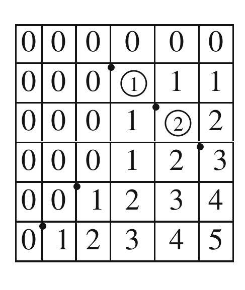
To make this visible, we usually put a $ \bullet$ into the matrix,
so that the permutation is encoded by the dots.
are the rank matrices corresponding to the longest element
$ w_0=4321$ and the identity element $ w=1234$, respectively. The encircled entries will be later called "pillar", these entries
determine the whole matrix, as explained in the next section. are the rank matrices corresponding to the four Coxeter elements in
$ S_4$: \begin{eqnarray*} s_1s_2s_3=2341, \quad s_1s_3s_2=2413, \quad s_2s_1s_3=3142, \quad s_3s_2s_1=4123, \end{eqnarray*} respectively. The Schubert varieties $ \X_{w_1}$ and $ \X_{w_2}$ are the only
singular Schubert varieties for $ n=4$. The smaller is the Schubert cell $ {\mathcal C}_w$, the bigger are the
numbers $ r_{ij}(w)$.
The rank matrix is completely determined by a few particular entries.
This idea is due to [Fulton1997] (see also [Woo2009], [Reiner et al.2011] and references therein). The
following notion is crucial for us.
We always encircle the pillar entries, in order to distinguish them.
In combinatorial terms, pillar entries can be characterized as follows.
An entry $ r_{ij}$ of a rank matrix $ r(w)$ is pillar if and only if
It worth noticing that, the more a given permutation $ w$ is
"close" to the identity, the more pillar entries the matrix $ r(w)$ has.
The matrix $ r(\Id)$ has $ n-1$ pillar entries $ r_{ii}=i$, for
$ 1\leq{}i\leq{}n-1$. The more $ w$ is "close" to the longest element
$ w_0$, the less pillar entries the matrix $ r(w)$ has. In
particular, $ r(w_0)$ is the only rank matrix with no pillar entries.
This statement is classical. For the sake of completeness, a proof will
be presented in Sect. 5.6. An explicit algorithm that reconstructs the
permutation $ w$ from the pillar entries of the rank
matrix $ r(w)$ will be presented in Sect. 4.2. Let us describe the pillar entries of the rank matrices corresponding to
the Coxeter elements.
Finally, the fact that the value of the pillar entry $ r_{i,i+1}$ (or
$ r_{i+1,i}$) is equal to $ i$ follows from (2.1).
⬜ We believe that the notion of pillar entry deserve a further study. In
particular, the number of pillar entries for a given permutation is an interesting
characteristic. Some of the basic properties of pillar entries will be presented in
Sect. 4.
Let us recall here Fulton's notion of essential entry. An entry
$ r_{ij}$ of a rank matrix $ r(w)$ is called essential
, see [Fulton1992] and also [Eriksson and Linusson1996], if It is proved in [Fulton1992] that every rank matrix (and therefore
the corresponding Schubert variety) is completely characterized by its essential
set. The notions of essential and pillar entries are somewhat
"complementary", as the inequality signs in formulas (2.3) and (2.4) are reversed,
cf. Appendix for a comparison.
The following conjecture asserts that if two Schubert varieties have the
same tangent cones, then they have the same number of pillars, whose values
are also the same, and whose position in the respective rank matrices can only
differ by transposition.
Example 2.1 and Proposition 2.8 are the first
examples that confirm our conjecture. We will give many other examples in
the sequel.
Note that the inverse of Conjecture 2.10 is false:
two permutations with partially transposed pillar entries do not necessarily
correspond to the same tangent cones.
Note however the following interesting inclusion: $ \T_{w'}\subset\T_w$.
Another restriction for partial transposition of pillars occurs more often
than the above discussed one. Given a permutation $ w$ and the
corresponding rank matrix $ r(w)$, then a partial transposition of the
pillar entries may not correspond to any rank matrix of any permutation.
It turns out that there are no rank matrices with the following pillar
entries:
Indeed, the above positions of pillar entries are impossible, since they
contradict formula (2.3), see also Sect. 4.1 for more
details. Let us briefly discuss the partial transpositions of linked pillar entries.
If one transpose some pillar entries of a rank matrix $ r(w)$, but not all
of them, then the following three possibilities may occur:
2.1. Rank Matrix.
![]()
\begin{equation}\label{Fulsps} r_{ij}=\#\{k\leq{}i\;\vert\; w(k)\leq{}j\}. \end{equation}
(2.1)
Example 2.1.
The rank matrices $ r(w)$
and $ r(w^{-1})$ are transposed to each other. In this case, one has:
\begin{eqnarray*} \T_w=\T_{w^{-1}}. \end{eqnarray*} This statement was conjectured (and checked for $ n\leq5$)
in [Eliseev and Panov2013]. However a short direct
proof can be easily given, see Sect. 5.7.
2.2. Permutation Diagram
![]()
Definition 2.2.
Given a permutation $ w \in S_{n}$, the
diagram of
$ w$ is defined with the following convention. In an $ (n+1)\times(n+1)$
grid, with row and columns numbered form $ 0$ to $ n$,
we place a dot in the upper left corner of the cell with coordinates
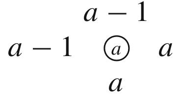
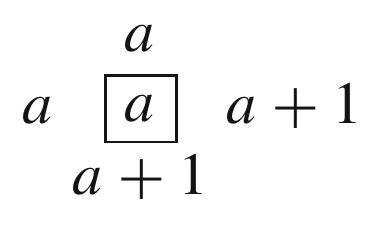
$ (i,j)$ whenever $ j=w(i)$. Proposition 2.3.
If the rank matrix $ r(w)$ is locally as
follows: \begin{eqnarray*} \begin{array}{c|c} a&a\\ \hline a&\!{}^{{}^\bullet}a+1 \end{array} \end{eqnarray*} where $ a+1$ is the value in position
$ (i,j)$, then the permutation $ w$ sends $ i$ to
$ j$.
Proof.
This readily follows from (2.1).
⬜
Example 2.4.
Consider the case of dimension $ 4$.
Example 2.5.
For the maximal cell $ {\mathcal C}_{w_0}$, the rank
matrix is given by: \begin{eqnarray*} r_{ij}(w_0)= \max\{0,\,i+j-n\}. \end{eqnarray*}
2.3. The Pillar Entries.
![]()
Definition 2.6.
An entry $ r_{ij}$ of a rank matrix
$ r(w)$ is called pillar
if it satisfies the conditions
\begin{equation}\label{LocPil} \left\{ \begin{array}{l} r_{ij}=r_{i-1,j}+1=r_{i,j-1}+1,\\ r_{ij}=r_{i+1,j}=r_{i,j+1}. \end{array} \right. \end{equation}
(2.2)
\begin{equation}\label{ComPil} \left\{ \begin{array}{ll} w(i)\leq{}j,&w(i+1)> j,\\ w^{-1}(j)\leq{}i,&w^{-1}(j+1)> i. \end{array} \right. \end{equation}
(2.3)
Proposition 2.7.
Every Schubert cell is completely determined by
the pillar entries of the rank matrix. Proposition 2.8.
The rank matrix of any Coxeter element of
$ S_n$ has $ n-2$ pillar entries \begin{eqnarray*} r_{i,i+1}=i, \quad\hbox{or}\quad r_{i+1,i}=i, \end{eqnarray*} for each
$ i\in\{1,2,\ldots,n-2\}$.
Proof.
Consider a Coxeter element $ w=\cdots\,s_i\,\cdots\,s_{i+1}\,\cdots{}$. It can be deduced directly
from (2.3),
that the entry $ r_{i,i+1}$ of $ r(w)$ is, indeed, a pillar entry.
Similarly, for a Coxeter element of the form $ w=\cdots\,s_{i+1}\,\cdots\,s_{i}\,\cdots{}$, one has that the
entry $ r_{i+1,i}$ is pillar. Similar arguments show that the rank matrix of
a Coxeter element cannot have other pillar entries than the above
$ n-2$ ones.
Remark 2.9.
In other words, the rank matrix of every
Coxeter element of $ S_n$ is determined by a sequence of
$ n-2$ inclusions: \begin{eqnarray*} V_i\subset{}\Csps^{i+1}, \quad\hbox{or}\quad \Csps^i\subset{}V_{i+1}, \end{eqnarray*} for $ i\in\{1,\ldots,n-2\}$. The $ 2^{n-2}$
Coxeter elements correspond to an arbitrary choice of one of the above
inclusions for every $ i$.
2.4. Fulton's Essential Entries
![]()
\begin{equation}\label{ComEss} \left\{ \begin{array}{ll} w(i)> j,&w(i+1)\leq{}j,\\ w^{-1}(j)> i,&w^{-1}(j+1)\leq{}i. \end{array} \right. \end{equation}
(2.4)
2.5. Transposed Pillars: The Main
Conjecture
![]()
Conjecture 2.10.
Given two permutations, $ w$ and
$ w'\in{}S_n$, if $ \T_w=\T_{w'}$ then the rank matrices $ r(w)$
and $ r(w')$ have the same number of pillar entries, and for every pillar
entry $ r_{ij}$ of $ r(w)$, one has the following alternative:
2.6. Restrictions: Forbidden
Transpositions
![]()
Example 2.11.
The simplest counterexample to the converse
statement that we know is provided by the following permutations
in $ S_6$: $ w=456321$ and $ w'=546132$. Indeed, the corresponding
rank matrices are (Fig. 1): respectively. The pillar entries are (partially)
transposed, but the permutations have different length: $ \ell(w)=12$ and
$ \ell(w')=11$, so that their tangent cones have different dimensions, and
cannot coincide.
Example 2.12.
Consider the permutation $ w=34521$ in
$ S_5$. The corresponding rank matrix is as follows:
2.7. More on Partial Transpositions
![]()
In view of Conjecture 2.10 and the above discussion, the main goal of
this paper is to investigate which (partial) transpositions of pillar entries of a
rank matrix $ r(w)$ lead to a new permutation $ w'$ and do
not change the tangent cone.
3.
Admissible Partial Transpositions: the Main Theorem
In this section we describe classes of permutations in $ S_n$ with identical tangent cones. Given a permutation $ w$, we define a series of operations called "admissible partial transpositions" and an equivalence class in $ S_n$ that consist of permutations related by such transpositions. We formulate our main result that all permutations from such a class correspond to the same tangent cone.
However, the described classes are not maximal. Examples in the end
of the section show that there are more permutations with identical tangent
cones.
We define an equivalence relation on the set of pillar entries of a rank
matrix. Roughly speaking, two pillar entries are in the same class if they are
"close enough" to each other.
It is convenient to display the linking relations between the pillar entries
using a graph.
For instance, Example 3.2 corresponds to the following graph (Fig. 5)
The connected components of the linking graph correspond to the
classes of linked pillar entries.
An admissible partial transposition
is an operation defined on rank matrices and on the group $ S_n$.
Roughly speaking, it consists in transposition of a part of the pillar entries,
such that linked pillar entries transpose (or not) simultaneously. More
precisely, we have the following:
In this section we formulate a sufficient condition for the tangent cones
of two Schubert varieties to coincide. Furthermore, it turns out that every
partial transposition of the pillar entries in the associated rank matrices defines
an operation on the group $ S_n$. Our main result is the following
We will prove this theorem in Sects. 4.5 and 5.7.
We will give an explicit description of the corresponding tangent cone
in Sect. 5.3. Note also that the Schubert varieties
corresponding to the Coxeter elements are smooth. Therefore, Corollary
3.8 can also
be deduced from the theorem of Lakshmibai, see [Lakshmibai1995] that describes the Zariski tangent
space.
Theorem 3.6 provides large classes of Schubert varieties
with identical tangent cones. However, these classes can be yet larger. In fact,
there are other cases of partial transposition of pillar entries than those
considered above.
This example is not covered by Theorem 3.6 and shows its
limits. For instance, it shows that the converse statement to Part (ii) of the
theorem is false. Existence of such partial transpositions of pillar entries
constitutes the main difficulty in solving the initial classification problem.
3.1. Linked and Dissociated Pillar Entries
![]()
Definition 3.1.
Example 3.2.
The following rank matrix (in which we omit
the extremal rows and columns) corresponding to the permutation
$ w=12,2,9,7,6,4,10,5,3,11,1,8\in S_{12}$ (Fig. 4):
have three classes of linked pillar entries (Fig. ExinS12): \begin{eqnarray*} \{r_{22}=1\}, \;\{r_{64}=2\},\; \{r_{67}=4, \,r_{69}=5, \,r_{97}=6, \,r_{9,10}=8, \,r_{11,7}=7\}. \end{eqnarray*}
3.2. The Linking Graph of Pillar Entries
![]()
Definition 3.3.
The linking
graph
is defined as follows.
3.3. Admissible Partial
Transpositions.
![]()
Definition 3.4.
Two rank matrices, $ r(w)$ and
$ r(w')$, are admissibly partially transpose
to each other if there exists a set $ \Lc$ which is a union of classes of
linked pillar entries for $ r(w)$, such that the set of pillar entries of
$ r(w')$ is as follows
\begin{equation}\label{ParTrEq} \left\{ \begin{array}{rcllll} r_{ij}'&=&r_{ij},& & \text{whenever} &r_{ij} \not\in \Lc,\\ r_{ji}'&=&r_{ij},& & \text{whenever} &r_{ij} \in \Lc.\\ \end{array} \right. \end{equation}
(3.1)
Example 3.5.
The permutation $ w=11,2,9,8,6,4,5,12,3,7,10,1$ in
$ S_{12}$ corresponding to the rank matrix (Fig. 6) is admissibly
partially transpose to the permutation given in Example 3.2. Indeed, the
set of pillar entries is the same except for the last connected component of the
graph, for which the positions of the pillar entries are transposed.
3.4. Statement of the Main
Theorem.
![]()
Theorem 3.6.
Example 3.7.
The Coxeter elements of $ S_4$, see
Example 2.4,
have the same two dissociated pillar entries, $ 1$ and $ 2$,
and their positions in the rank matrices differ by transpositions. Therefore, the
Schubert varieties corresponding to these elements have the same tangent cone.
This statement can be generalized, see below Corollary 3.8.
Schubert varieties corresponding to the Coxeter
elements have the same tangent cone.
Proof.
The pillar entries of Coxeter elements are dissociated and differ by
partial transpositions; see Proposition 2.8.
⬜
3.5. Other Admissible Transpositions
![]()
Example 3.9.
The permutations $ w=6745321$ and
$ w'=6753421$ in $ S_7$ have the following rank matrices (Fig. 7): The
rank matrix $ r(w)$ has two pillar entries: $ r_{16}$ and
$ r_{34}$, the interval $ [3,4]$ is entirely contained in the interval
$ [1,6]$. Therefore, these pillar entries of $ w$ are related in
view of Definition 3.1. However, it is easy to check that
$ \T_w=\T_{w'}$, in other words, the partial transposition relating $ w$
and $ w'$ should also be considered as admissible. 
4. Combinatorial Aspects of Rank
Matrices and Pillar Entries
In this section we describe the main properties of pillar entries of rank matrices and develop the technique necessary from the proof of our main result.
Recall that the set of pillar entries of a rank matrix $ r(w)$ determines the permutation $ w$ (see Proposition 2.7). We present two algorithms: that of reconstruction of $ w$ from the pillar entries of $ r(w)$, and that of calculating the permutation of $ w'$ obtained by some partial transpositions of pillar entries of $ r(w)$. This allows us to prove Part (i) of Theorem 3.6.
We also give an explicit formula for the (co)dimension of the Schubert
cell $ {\mathcal C}_w$ in terms of the pillar entries of the rank matrix $ r(w)$.
This result can be useful for the further study of combinatorics of rank matrices.
The rank matrix $ r(w)$ is determined by the diagram of the
corresponding permutation $ w$.
The positions of the pillar entries in $ r(w)$ can be determined
by local structure of the diagram of $ w$. Consider horizontal strips of
height $ 1$ and a vertical strips of width $ 1$ in the diagram,
such that the upper left and the lower right corners are marked dots of the
permutation:
It will be useful in the sequel to have the following observation.
The proof of the vice-versa statement is the same, with the coordinates
of every marked dot switched. ⬜ In this section we present an algorithm of constructing the diagram of
$ w$ from the set of pillar entries. Let us introduce some useful notation. First we numerate the pillar
entries in the lexicographical order, that is, from left to right in each row and
then counting the rows from top to bottom. Then we set:
$ (p_i,q_i)=$ the position of the $ i$-th pillar;
$ K_i=r_{p_iq_i}(w)=$ the value of the $ i$-th pillar entry;
$ NW_i=$ The North-west region of the $ i$-th pillar entry.
We draw the $ (n+1)\times(n+1)$ square grid; columns and rows of this
grid are separated by $ n$ horizontal lines and $ n$ vertical
lines. We mark the given pillar entries in $ N$ cells of the grid (thus,
$ N$ is the number of pillar entries). Our permutation $ w$
will appear as a set of $ n$ dots in the intersections of horizontal and
vertical lines, one on each horizontal line and one on each vertical line. The diagram of $ w$ is constructed in $ N+1$ steps.
At every step, we place some dots into the interior of the region $ NW_i$.
If the action requested at any step is impossible by any reason, then our set of
"pillar entries" is not the set of pillar entries of $ r(w)$ for any
$ w$. For $ i=1,\dots,N$, at the $ i$-th step, we fist count the
number of dots placed in the interior of $ NW_i$ at the previous steps. If
this number is $ L$, we need to add $ k_i=K_i-L$ dots into
\begin{eqnarray*} NW_i-(NW_1\cup\dots\cup NW_{i-1}). \end{eqnarray*} For this, we numerate the horizontal and vertical lines within
$ NW_i$ which do not bear any of the $ L$ dots placed at the
previous steps, respectively from bottom to tor and from right to left. Then,
for $ j=1,\dots,k_i$ we place a dot at the intersections of the vertical line
number $ j$ and the horizontal line number $ k_i+1-j$
(Fig. 9).
Our algorithm requests that neither of these dots falls into any of the
regions $ NW_1,\dots,NW_{i-1}$. The final, $ (N+1)$-st step works according the same rules with
the whole matrix playing the role of $ NW_{N+1}$. The above algorithm is the only way to mark dots without creating
an extra pillar or changing the values of the pillar entries. Note that, for the
Fulton essential set, a reconstruction algorithm is given in [Eriksson and Linusson1996].
The dimension and codimension of a Schubert cell $ {\mathcal C}_w$ (or a
Schubert variety $ \X_w$) can be computed directly form the set of pillar
entries of the corresponding rank matrix $ r(w)$. The number \begin{eqnarray*} \codim({{\mathcal C}_w})=\ell(ww_0)=\#\{i< j : w(i)< w(j)\} \end{eqnarray*} can be obtained in the diagram of
$ w$ counting the intersections of the horizontal segments and the
vertical segments of the grid that are at the right and above each dots,
respectively: The following formula gives the codimension of a Schubert cell from
the data of its pillar entries.
Given a permutation of $ w\in{}S_{n}$, we will show the existence of
permutations whose pillar entries form the subsets in the set of pillar entries
of $ r(w)$ obtained by removing of some classes of linked pillar entries.
The pillar entries of $ r(w)$ are decomposed in the disjoint
union of classes of linked pillar entries: $ \{r_{ij}(w)\}=\Lc_{1}\sqcup \Lc_{2}\sqcup \ldots \sqcup \Lc_{s}.$ These classes correspond
to subintervals $ I_1,I_2,\ldots,I_s$ of the interval $ [0,n]$; these subintervals
have integer endpoints and pairwise have no interior points. The class
$ \Lc_t$ corresponds to the interval $ I_t$, if, for every
$ r_{ij}(w)\in\Lc_t$ both $ i$ and $ j$ belong to $ I_t$.
We order the intervals $ I_t$, from the left to the right, and order the
classes $ \Lc_t$ accordingly. Consequently, if $ u< v$ and
$ r_{ij}(w)\in \Lc_{u},\,r_{i'j'}(w)\in \Lc_{v}$, then $ i\leq{}i',\,i\leq{}j',j\leq{}i',\,j\leq{}j'$. In particular, for $ u< v$, all pillar
entries from $ \Lc_{u}$ lexicographically precede the pillar entries from
$ \Lc_{v}$. The following statement is our first application of the reconstruction
algorithm presented in Sect. 4.2.
The lexicographic order suggests a natural series of admissible partial
transpositions, such that all the classes of linked pillar entries $ \Lc_i$
transpose for $ i$ less or equal to some value. In this section we
present en explicit algorithm of calculating the resulting permutations. This
algorithm is the main ingredient of the proof of Part (i) of Theorem 3.6. For $ t\in \{1, \ldots, s\}$, we define the
elementary partial transposition
$ w'=\trp_{t}(w)$, as the permutation having the following set of pillar entries:
\begin{eqnarray*} \left\{ \begin{array}{rclll} r_{ji}(w')&=&r_{ij}(w), & \text{if} &r_{ij}(w) \in \Lc_{1}\sqcup \ldots \sqcup \Lc_{t};\\ r_{ij}(w')&=&r_{ij}(w), & \text{if} &r_{ij}(w) \in \Lc_{t+1}\sqcup \ldots \sqcup \Lc_{s}.\\ \end{array} \right. \end{eqnarray*} Note that every partial transposition can be obtained as a
sequence of elementary partial transpositions. Given a permutation $ w=w_1w_2\ldots{}w_n\in{}S_n$, the entries $ w_k$ of
$ w$ are separated into two disjoint groups, $ I_1\sqcup{}I_2$:
\begin{eqnarray*} \left\{ \begin{array}{rclll} w_k\in{}I_1,& \text{if}&k\leq{}\max(j), & \text{for pillars} &r_{ij}(w) \in \Lc_{1}\sqcup \ldots \sqcup \Lc_{t};\\ w_k\in{}I_2,& \text{if}&k> {}\min(i), & \text{for pillars} &r_{ij}(w) \in \Lc_{t+1}\sqcup \ldots \sqcup \Lc_{s}.\\ \end{array} \right. \end{eqnarray*} The algorithm of calculation the permutation $ w'=w'_1w'_2\ldots{}w'_n$,
obtained via the above elementary partial transposition, consists in three
steps: The proof of the above algorithm is straightforward.
is obtained into three steps: \begin{eqnarray*} 2\,3\,\vert\,4\,1 \quad\to\quad 2\,.\,\vert\,4\,. \quad\to\quad .\,1\,\vert\,4\,. \quad\to\quad 3\,1\,\vert\,4\,2, \end{eqnarray*} so that $ w'=3142$ is
another Coxeter element, already considered in Example 2.4, b).
For every $ w\in{}S_n$, the above algorithm implies the existence of
a permutation $ w'$ such that the pillar entries of $ r(w')$ are
obtained by an admissible partial transposition of pillar entries of $ r(w)$.
Part (i) of Theorem 3.6 is proved.
4.1. Rank Matrix and Its Pillar
Entries from the Permutation Diagram.
![]()
Proposition 4.1.
One has the following formula:
\begin{equation}\label{dots} r_{ij}(w)=\#\{\text{dots in the upper left quadrant from the cell } (i,j)\}. \end{equation}
(4.1)
Proof.
This readily follows from (2.1).
⬜
Proposition 4.2.
Every pillar is located at the intersection of a
horizontal strip of height $ 1$ and a vertical strip of
width $ 1$.
Proof.
This is a direct consequence of (2.3).
⬜
Example 4.3.
Rank matrix and its pillar entries of
$ w=853471692$ in $ S_9$ is as follows (Fig. 8).
Proposition 4.4.
Every horizontal strip of height $ 1$
necessarily intersects with a vertical strip of width $ 1$, and
vice-versa.
Proof.
Let $ (i,j),\;(i+1,j+k)$, $ k> 0$, be the marked dots of a horizontal
strip of height one. If $ k=1$, then our horizontal strip is also a vertical
strip, and these two (identical) strips intersect each other. Let $ k> 1$,
and let $ (i_1,j+1),\,\ldots,\,(i_{k-1},j+k-1)$ be the marked dots of the diagram of $ w$,
lying on the vertical lines crossing our strip; neither of $ i_1,\,\ldots,i_{k-1}$ is
$ i$ or $ i+1$. If $ i_1> i+1$, then the vertical strip with
marked dots $ (i,j),\,(i_1,j+1)$ intersects our horizontal strip. Similarly, if
$ i_{k-1}< i$, then the vertical strip with marked dots $ (i_{k-1},j+k-1),\;(i+1,j+k)$
intersects our horizontal strip. If $ i_1< i$ and $ i_{k-1}> i+1$, then for
some $ s$, $ i_s< i$ and $ i_{s+1}> i+1$. In this case, the
vertical strip with marked dots $ (i_s,j+s),\,\ldots,\,(i_{s+1},j+s+1)$ intersects our horizontal strip.
4.2. Reconstructing
$ w$ from the Pillar Entries of $ r(w)$.
![]()
Example 4.5.
Figure 10 below illustrates our algorithm for
$ w=853471692\in{}S_9$. At each step we color the North-West region at the pillar. The
dark grey part of the region intersects with North-West regions at previous
pillar entries; the light grey part is the area where the new dots are placed.
Example 4.6.
Given positive integers, $ i,j,a$
satisfying the conditions: \begin{eqnarray*} a\leq{}i,j\leq{}n, \quad i+j-a< n, \end{eqnarray*} there exists an element, $ w_{i,j,a,n}\in{}S_n$,
whose rank matrix has the unique pillar entry $ r_{ij}=a$. The above
algorithm immediately gives: \begin{eqnarray*} w_{i,j,a,n}&=&(n,n-1,\ldots,n+1-i+a,j,j-1,\ldots,j-a+1,n-i \\ &&+\,a,n-i+a-1,\ldots,j+1,j-a,j-a-1,\ldots,1). \end{eqnarray*} This element appeared in [[Reiner et al.2011], Corollary 4.5]. Remark 4.7.
If one defines the following partial ordering on
the set of ordered pillar entries \begin{eqnarray*} j\prec i &\Longleftrightarrow& \text{the }j\text{-th pillar lies in the region at the North-West of the }i\text{-th pillar}\\ &&\text{i.e. } j< i \text{ , } p_j\leq p_i \text{ and } q_j\leq q_i \end{eqnarray*} one can write the following relation
between the $ K_{i}$'s and $ k_{i}$'s \begin{eqnarray*} K_{i}=k_{i}+\sum_{j\prec i} k_{j}. \end{eqnarray*}
4.3. (Co)dimension from the Set of Pillar
Entries
![]()
\begin{equation} \label{codimcross} \codim({{\mathcal C}_w})=\#\{\text{crosses in the diagram of }w\}, \end{equation}
(4.2)
Theorem 4.8.
Using the notation of Sect. 4.2 one computes
\begin{eqnarray*} \codim({{\mathcal C}_w})=\sum_{i=1}^N\, k_i\; (K_i+n-p_i-q_i). \end{eqnarray*}
Proof.
This formula is obtained using the reconstruction algorithm of
$ w$ from the set of pillar entries (see Sect. 4.2) and
(4.2)
. For each dot in the diagram of $ w$, we count the crosses on the
horizontal segment at its right. At step $ i$ of the construction, the
$ k_i$ new dots will contribute with the same number of crosses in
(4.2)
. The reconstruction algorithm of $ w$ implies that these crosses can
be produced only by the dots that are located at the South-East of the
$ i$-th pillar (otherwise it would contradict the fact that one uses
the closest available vertical lines at the left of the $ i$-th pillar).
The number of dots in the South-East area is easy to compute from our data:
\begin{eqnarray*} \begin{array}{rcl} \#\{\text{dots at SE}\}&=& \#\{\text{dots}\}-\#\{\text{dots at NW}\}-\#\{\text{dots at NE}\}-\#\{\text{dots at SW}\}\\ &=&n-K_i-(p_i-K_{i})-(q_i-K_i)\\ &=&K_i+n-p_i-q_i. \end{array} \end{eqnarray*} Hence the result. ⬜
4.4. Truncated Permutation
![]()
Proposition 4.9.
For every $ t\in \{1, \ldots, s\}$ there exists a unique
permutation, denoted $ \tr_{t}(w)$, having $ \Lc_{1}\sqcup \Lc_{2}\sqcup \ldots \sqcup \Lc_{t}$ as set of pillar
entries.
Proof.
This permutation is obtained by stopping the algorithm of
reconstruction of $ w$ given in Sect. 4.2 after the step
corresponding to the last pillar of the class $ \Lc_{t}$ and jumping to the
final step. ⬜
Example 4.10.
For $ w=(12,2,9,7,6,4,10,5,3,11,1,8)$ as in Example 3.2, the classes are
numbered as follows
\begin{eqnarray*} \Lc_{1}=\{r_{22}=1\}, \;\Lc_{2}=\{r_{64}=2\},\; \Lc_{3}=\{r_{67}=4, \,r_{69}=5, \,r_{97}=6, \,r_{9,10}=8, \,r_{11,7}=7\}. \end{eqnarray*}One then obtains the truncated permutations
\begin{eqnarray*} \tr_{1}(w)=(12, 2, 3, 11, 10, 9, 8, 7, 6, 5, 4, 1), \quad \tr_{2}(w)=(12, 2, 11, 10, 9, 4, 8, 7, 6, 5, 3, 1). \end{eqnarray*}
4.5. Elementary Partial
Transpositions.
![]()
Example 4.11.
For the Coxeter element $ w=2341\in{}S_4$, the
elementary transposition
5.
Proof of the Main Theorem
In this section, we prove Proposition 2.7 and Part (ii) of
Theorem 3.6.
In the neighborhood of the standard flag $ F_0$, the flag
variety $ \F$ is identified with the subgroup of unitriangular matrices
Our next goal is to describe the Schubert cells and Schubert varieties
in terms of this coordinate system.
Let $ M_{ij}$ be the $ (n-j)\times{}i$ submatrix of $ X$
consisting of the last $ n-j$ rows and the first $ i$ columns.
The following lemma translates the description of Schubert cells in
terms of rank matrices into an algebraic descripition in the above coordinate
system.
The Schubert variety $ \X_w$ is determined, in a neighborhood
of the standard flag $ F_0$, by a system of polynomial equations in the
variables $ x_{ij}$. The equations are obtained as follows. For each
couple of indices $ i, j$, formula
(5.2)
leads to a set of equations that expresses the annihilation of the minors of the
matrix $ M_{ij}$ of size larger than its rank. From Proposition 2.7, it suffices to
consider only the equations for the indices $ i,j$ corresponding to a
pillar entry $ r_{ij}(w)$ in the rank matrix of $ \X_w$. The system of equations of the tangent cone $ \T_w$ of
$ \X_{w}$ is obtained, roughly speaking, as the homogeneous lower degree
parts of the equations of $ \X_w$. More precisely, the equations of
$ \X_w$ can be written in such a way that the homogeneous terms of
lower degree are linearly independent. Then the system of $ \T_w$ is
obtained by removing all of the monomials of higher degree in the equations of
$ \X_w$.
so that the Schubert cell $ {\mathcal C}_{w}$ is determined by the
condition $ \dim(V_{2}\cap{}\Csps^{2})=1$, that translates in coordinates as the condition that a
certain linear combination of two first column vectors belong to the subspace
$ \Csps^{2}$, i.e., the matrix $ M_{22}$ degenerates. The tangent cone $ \T_{w}$ is $ 5$-dimensional,
whereas the Zariski tangent space is the whole $ 6$-dimensional
tangent space $ T_{F_{0}}\F$. In the case $ i\leq{}j$, the minors of $ M_{ij}$ are
homogeneous polynomial expressions. The following observation explains the
reason for which two pillar entries transposed to each other, in many situation
give the same contribution to the system of equation of the tangent cones.
If $ i> j$, then $ M_{ji}$ is the complement of the upper
right square submatrix in $ M_{ij}$ (of size $ i-j$) with
$ 1$'s on the diagonal: \begin{eqnarray*} M_{ij}= \left( \begin{array}{ll|ccc} &&1&\\ &&\vdots&\ddots\\ &&&\cdots&1\\ \hline &M_{ji}\\ \end{array} \right). \end{eqnarray*} The lower degree homogeneous
part in the expression of any minors of $ M_{ij}$ of size $ r\geq i-j$
involving the last $ i-j$ columns corresponds precisely to a minor of
$ M_{ji}$ of size $ r-i+j$, and vice versa.
Let us show that the pillar entries determine the rank matrix. We use
the fact that the rank matrix $ r(w)$ completely determines the Schubert
variety $ \X_{w}$. For a permutation $ w$, let $ r_{i_1j_1},\ldots,r_{i_Nj_N}$ be the pillar
entries of the matrix $ r(w)$ and let $ C_{ij}$ be the condition
\begin{eqnarray*} \rank(M_{ij})\le i-r_{ij}(w) \end{eqnarray*} from the system of conditions determining the Schubert variety
$ \X_{w}$ (see Sect. 5.3). There are obvious implications:
If
$ r_{i+1,j}=r_{ij}$, then
$ C_{ij}$ implies
$ C_{i+1,j}$;
If
$ r_{i+1,j}=r_{ij}+1$, then
$ C_{i+1,j}$ implies
$ C_{ij}$;
If
$ r_{i,j+1}=r_{ij}$, then
$ C_{i,j}$ implies
$ C_{i,j+1}$;
If
$ r_{i,j+1}=r_{ij}+1$, then
$ C_{i,j+1}$ implies
$ C_{ij}$. Let us visualize the matrix $ [C_{ij}]$ as an $ (n+1)\times(n+1)$ grid
and show the above implications by arrows between the neighboring cells; the
resulting diagram for the matrix from Example 2.12 is shown
below (Fig. 12).
Take any cell of the grid and trace a path from it in the following way:
we move in the direction opposite to the arrow. If there arises a choice of several
such direction, choose any of them. If there is no such directions, then stop. It
is important that our path never passes through a cell more that once: when
we move right or upward, the entry stays unchanged, when we move left or
downward, the entry grows (by one at a step). To move from a cell back to the
same cell, we have to make at least one move left of downward, and the entry
cannot remain unchanged. Thus our path leads from our (arbitrarily chosen)
cell to either a pillar or to a corner cell. Moving along this path in the opposite
direction, we show that every condition $ C_{ij}$ follows either from one
of the pillar conditions $ C_{i_1j_1},\dots,C_{i_Nj_N}$ or one of the conditions $ C_{0 0}, C_{nn}$,
which are empty. Thus, the Schubert variety $ \X_{w}$ is determined by
the conditions $ C_{i_1j_1},\dots,C_{i_Nj_N}$, that is, determined by the pillars. To illustrate the above technique, let us calculate the tangent cone of
the Schubert varieties corresponding to the Coxeter elements explicitly.
We will need the following lemma We are grateful to M.
Kashiwara for a simple proof. ×
1.
We are ready to prove Theorem 3.6, Part (ii).
Assume that two permutations, $ w$ and $ w'$, are
admissibly partially transpose to each other. We want to show that the
tangent cones of $ \X_{w}$ and $ \X_{w'}$ coincide. We can assume that $ w'=\trp_{t}(w)$ is an elementary partial
transposition of $ w$, see Sect. 4.5 for the
definition and the notation. The systems of equations for $ \X_{w}$ and
$ \X_{w'}$ split in two parts: the equations coming from the pillar entries
in the classes $ \Lc_{1}\sqcup \ldots \sqcup \Lc_{t}$ (these equations are a priori different for
$ w$ and $ w'$ since the pillar entries are not in the same
positions) and the equations coming from the pillar entries in the other classes,
namely in $ \Lc_{t+1}\sqcup \ldots \sqcup \Lc_{s}$. The latter equations are identically the same for
$ w$ and $ w'$. Consider finally the two subsystems of equations for $ \X_{w}$ and
$ \X_{w'}$ coming from the pillar entries in the set $ \Lc_{1}\sqcup \ldots \sqcup \Lc_{t}$. These
two subsystems are precisely those describing the Schubert varieties associated
to $ \tr_{t}(w)$ and $ \tr_{t}(w')$, respectively. These two varieties have same
tangent cones since $ \tr_{t}(w)=\tr_{t}(w')^{-1}$. After intersecting with the tangent cone of
the variety described by the rest of the system, one therefore obtains the same
tangent cone for $ \X_{w}$ and $ \X_{w'}$. Theorem 3.6 is proved.
5.1. A Coordinate System
![]()
\begin{equation}\label{CoOrdEq} X= \left( \begin{array}{cccc} 1&&&\\ x_{21}&1&\\ \vdots&\ddots&\ddots\\ x_{n1}&\cdots&x_{n\,n-1}&\!\!1 \end{array} \right) \end{equation}
(5.1)
5.2. Submatrices.
![]()
5.3. Relation to the Rank
Matrices.
![]()
Lemma 5.1.
The matrix $ X$ represents a flag in
the Schubert cell $ {\mathcal C}_w$ if and only if
\begin{equation}\label{DimEq} \rank(M_{ij})= i-r_{ij}(w), \end{equation}
(5.2)
Proof.
The space $ \Csps^j$ consists of vectors with zeros at positions
$ \geq{}j+1$. One then has \begin{eqnarray*} j+\rank(M_{ij})=\dim(V_i+\Csps^j)=i+j-r_{ij}(w). \end{eqnarray*} Hence
(5.2)
. ⬜
5.4. Systems of Equations for
$ \X_{w}$ and $ \T_{w}$.
![]()
Example 5.2.
As we mentioned in Introduction, the first
example of a Schubert variety with singularity at the origin correspond to the
permutation $ w=4231\in{}S_{4}$ (see [Billey and Lakshmibai2000], [Lakshmibai and Sandhya1990]). Written in our
local coordinates: \begin{eqnarray*} \left( \begin{array}{llll} 1\\ x_{21}&1\\ x_{31}&x_{32}&1\\ x_{41}&x_{42}&x_{43}&1 \end{array} \right) \end{eqnarray*} the equation of the corresponding tangent cone
$ \T_{w}$ (the same as the equation of $ \X_{w}$) is: $ x_{31}x_{42}-x_{32}x_{41}=0$.
Indeed, the rank matrix of $ w$ is as follows:
5.5. The Duality.
![]()
5.6. Proof of Proposition 2.7
![]()
Proposition 5.3.
The tangent cone of the Schubert varieties
corresponding to the Coxeter elements of $ S_n$ is given by the
equations
\begin{equation}\label{CoxTVEq} x_{ij}=0, \quad\hbox{for}\quad i-j> 1. \end{equation}
(5.3)
Proof.
It was already proved that Schubert varieties corresponding to the
Coxeter elements have the same tangent cone, see Corollary 3.8. Let us consider
the particular Coxeter element \begin{eqnarray*} w=s_1s_2\,\cdots\,{}s_{n-1}=234\ldots{}n1. \end{eqnarray*} Its rank matrix has the following
pillar entries (cf. Proposition 2.8): \begin{eqnarray*} r_{12}=1,\quad r_{23}=2,\ldots,\quad r_{n-2,n-1}=n-2. \end{eqnarray*} By Lemma 5.1 and
Proposition 2.7, the Schubert variety $ \X_{w}$ is locally
determined by the conditions $ \rank(M_{ij})=0$, for $ i> j$. Therefore, in
the local coordinate system $ (x_{ij})$, the Schubert variety $ \X_{w}$,
and thus its tangent cone $ \T_w$, is a linear subspace given by
Eq. (5.3).
⬜
5.7. Proof of Theorem 3.6
![]()
Lemma 5.4.
For every $ w\in{}S_n$, the Schubert varieties
$ \X_{w}$ and $ \X_{w^{-1}}$ have same tangent cone.
Proof.
The homeomorphism $ x\mapsto x^{-1}$ from $ BwB$ to
$ Bw^{-1}B$ induces the isomorphism $ f\mapsto -f$ from $ \T_{w}$ to
$ \T_{w^{-1}}$. Since $ -f\in\T_w$ for every $ f\in\T_w$, this shows that
$ \T_{w^{-1}}=\T_{w}$. ⬜
6.
Enumerative Results
Theorems 3.6 gives an efficient method for calculating the number of different tangent cones of Schubert varieties. In this section, we give the result in small dimensions and codimensions. The general result is still out of reach.
Recall that the total number of Schubert varieties is $ n!$, the
total number of their tangent cones is smaller. It would be interesting to find
asymptotic of the number of tangent cones.
In the case $ n=4$, the comparative number of Schubert
varieties and their tangent cones, as a function of their dimension, is given by
the following table. \begin{eqnarray*} \begin{array}{r|c|c|c|c|c|c|c} \dim&0&1&2&3&4&5&6\\ \hline \hbox{Schub}&1&3&5&6&5&3&1\\ \hline \hbox{TangCones}&1&3&3&3&3&2&1 \end{array} \end{eqnarray*} The total number of tangent cones in this case
is $ 16$. For $ n=5$, the table is: \begin{eqnarray*} \begin{array}{r|c|c|c|c|c|c|c|c|c|c|c} \dim&0&1&2&3&4&5&6&7&8&9&10\\ \hline \hbox{Schub}&1&4&9&15&20&22&20&15&9&4&1\\ \hline \hbox{TangCones}&1&4&6&7&9&9&10&8&6&2&1 \end{array} \end{eqnarray*} The total number of
tangent cones is $ 63$. For $ n=6$, the distribution of the tangent cones is as follows:
\begin{eqnarray*} \begin{array}{r|c|c|c|c|c|c|c|c|c|c|c|c|c|c|c|c|c} \dim&0&1&2&3&4&5&6&7&8&9&10&11&12&13&14&15\\ \hline \hbox{TangCones}&1&5&10&14&20&25&31&36&40&40&34&24&15&8&3&1 \end{array} \end{eqnarray*} The total number of tangent cones for $ n=6$ is
$ 343$. For $ n=7$ and $ 8$, the total numbers of tangent
cones are: $ 1821$ and $ 13041$, respectively These
numbers are obtained using computer programs. × 2. Note that the sequence
$ 16,63,343,1821,13041,\ldots$ does not appear in Sloane's online Encyclopedia of Integer
Sequences.
Let us also consider the case of small codimension. The tangent cone of the Schubert variety $ \X_{w_0}$ corresponding
to longest element $ w_0\in{}S_n$, is the only one tangent cone of dimension
$ \frac{n(n-1)}{2}$. Next, in the case of dimension $ \frac{n(n-1)}{2}-1$ ( i.e.
, of codimension $ 1$), there are $ n-1$ Schubert varieties
that have $ \left[\frac{n}{2}\right]$ tangent cones. Indeed, the elements $ \X_w$
and $ \X_{w^{-1}}$ have the same tangent cone. There are $ \frac{(n+2)(n-1)}{2}$ Schubert varieties of codimension
$ 2$. The number of their tangent cones depend on the parity of
$ n$, as given by the following statement.
6.1. Low-Dimensional Cases
![]()
6.2. Tangent Cones of Codimension
$ 2$
![]()
Proposition 6.1.
The number of tangent cones of codimension
$ 2$ is: \begin{eqnarray*} 2+\frac{(n-3)(n+11)}{8}, \quad\hbox{and}\quad 3+\frac{(n-4)(n+14)}{8}, \end{eqnarray*} for odd $ n$, and for even
$ n$, respectively.
Proof.
A straightforward calculation.
⬜
Appendix 
A1 Comparison of Pillar
Entries to Essential Entries.
Below are a series of examples and comments about the relationship between pillar entries and Fulton's essential entries, see also [Woo2009]. Recall that essential entries are boxed (while pillar entries are encircled as above).
Let us consider examples that emphasize the difference between the notions of essential and pillar entries. The most interesting case is that of the Coxeter elements.
Example 6.2.
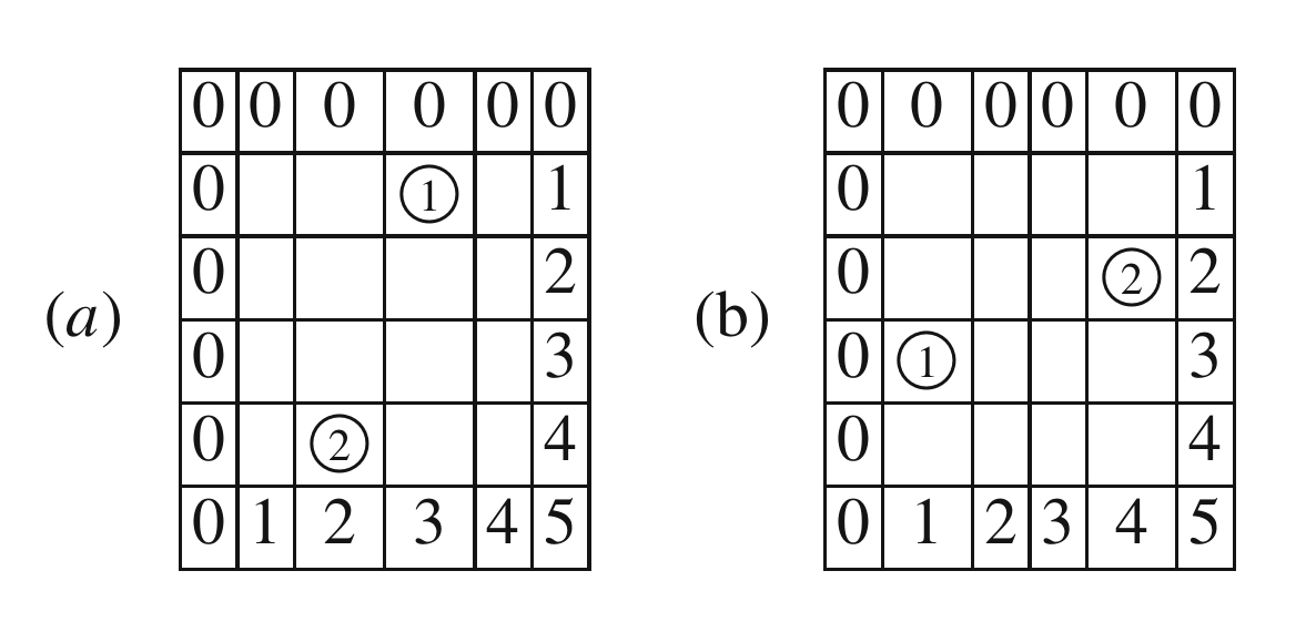
- (a) The rank
matrix of the element $ w_0=4\,3\,2\,1$ in $ S_4$ has three essential
entries
and no pillar entries. It can be deduced from formula (2.1), that, for an arbitrary $ n$, the only rank matrix without pillar entries is the matrix $ r(w_0)$ of the longest element $ w_0\in{}S_n$. This matrix has $ n-2$ essential entries along the antidiagonal.
- (b) For each of
the elements $ w_1=2\,1\,4\,3$ and $ w_2=4\,2\,3\,1$ of $ S_4$, we have two
essential entries and one pillar:
Note that the position of the pillar entry in the above matrices is the same, while those of the essential entries are different.
- (c) For the
Coxeter elements of $ S_{4}$, we have:
A2 Rothe Diagrams and
Opposite Rothe Diagrams.
The Rothe diagram ([Rothe1800]) of a permutation $ w\in S_{n}$ is an $ n\times{}n$ square table obtained according to the following rule. Dot the cell $ (i,j)$ whenever $ w(i)=j$, shade all the cells of the row at the right of the dotted cell and all the cells of the column below the dotted cell (including the dotted cell). Note that the length $ \ell(w)$ is equal to the number of white cells in the Rothe diagram.
It was noticed in [Fulton1992], that the white cells having a South and East frontier with the shaded region give the positions of the essential entries in the corresponding rank matrix. The value of an essential entry is equal to the number of dots in the upper left quadrant of the Rothe diagram with the origin at the corresponding cell. Let us explain a similar rule to obtain positions of pillar entries.
 The Rothe diagram gives the unique essential entry in the rank matrix:
$ r_{31}=0$, whereas the opposite diagram gives two pillar entries:
$ r_{12}=1$ and $ r_{23}=2$
The Rothe diagram gives the unique essential entry in the rank matrix:
$ r_{31}=0$, whereas the opposite diagram gives two pillar entries:
$ r_{12}=1$ and $ r_{23}=2$Consider the opposite Rothe diagram obtained with the following rule. Shade all the cells of the row strictlty at the left of the dotted cell and all the cells of the column strictly above the dotted cell (the dotted cell is not shaded). Note that the number of white undotted cells in the opposite Rothe diagram is equal to $ \ell(w)$ (Table 1).
It follows directly from Definition 2.6, that the white cells having a South and East frontier with the shaded region in the opposite Rothe diagram give the positions of the pillar entries in the corresponding rank matrix. The value of a pillar entry is equal to the number of dots in the upper left quadrant of the diagram.
Acknowledgements.
This work was started during our stay at the American Institute of Mathematics within the research program SQuaRE. The final version was completed during a RiP stay at the Mathematisches Forschungsinstitut Oberwolfach. We are grateful to AIM and MFO for their hospitality. We are also grateful to M. Kashiwara and A. Panov for helpful discussions, and to the referee for his/her helpful comments. S. M-G. was partially supported by the ANR project SC$ ^{3}$A, ANR-15-CE40-0004-01.References
[Billey and Lakshmibai2000] Billey, S., Lakshmibai, V.: Singular Loci of Schubert Varieties. Progress in Mathematics, vol. 182. Birkhäuser Boston, Inc., Boston (2000)
[Bochkarev et al.2016] Bochkarev, M., Ignatyev, M., Shevchenko, A.: Tangent cones to Schubert varieties in types $ A_n$, $ B_n$ and $ C_n$. J. Algebra 465 , 259–286 (2016)
[Brion2005] Brion, M.: Lectures on the Geometry of Flag Varieties, Topics in Cohomological Studies of Algebraic Varieties, pp. 33–85. Trends Math, Birkhäuser, Basel (2005)
[Carrell and Kuttler2006] Carrell, J., Kuttler, J.: Singularities of Schubert varieties, tangent cones and Bruhat graphs. Am. J. Math. 128 (1), 121–138 (2006)
[Eliseev and Panov2013] Eliseev, D., Panov, A.: Tangent cones of Schubert varieties for $ A_n$ of low rank. J. Math. Sci. (N. Y.) 188 (5), 596–600 (2013)
[Eriksson and Linusson1996] Eriksson, K., Linusson, S.: Combinatorics of Fulton's essential set. Duke Math. J. 85 , 61–76 (1996)
[Fulton1992] Fulton, W.: Flags, Schubert polynomials, degeneracy loci, and determinantal formulas. Duke Math. J. 65 , 381–420 (1992)
[Fulton1997] Fulton, W.: Young Tableaux. With Applications to Representation Theory and Geometry. London Mathematical Society Student Texts, vol. 35. Cambridge University Press, Cambridge (1997)
[Ignatyev and Shevchenko2015] Ignatyev, M., Shevchenko, A.: On tangent cones to Schubert varieties in type $ D_n$. St. Petersbourg Math. J. 27 , 28–49 (2015)
[Kirillov1995] Kirillov, A.A.: Variations on the triangular theme. In: Lie Groups and Lie Algebras: E. B. Dynkin's Seminar, volume 169 of Amer. Math. Soc. Transl. Ser. vol. 2, pp. 43–73. American Mathematical Society, Providence (1995)
[Lakshmibai1995] Lakshmibai, V.: Tangent spaces to Schubert varieties. Math. Res. Lett. 2 (4), 473–477 (1995)
[Lakshmibai and Sandhya1990] Lakshmibai, V., Sandhya, B.: Criterion for smoothness of Schubert varieties in $ Sl(n)/B$. Proc. Indian Acad. Sci. Math. Sci. 100 (1), 45–52 (1990)
[Panov2015] Panov, A.N.: Invariants of the coadjoint action on the basic varieties of the unitriangular group. Transform. Groups 20 (1), 229–246 (2015)
[Polo1994] Polo, P.: On Zariski tangent spaces of Schubert varieties, and a proof of a conjecture of Deodhar. Indag. Math. (N.S.) 5 (4), 483–493 (1994)
[Reiner et al.2011] Reiner, V., Woo, A., Yong, A.: Presenting the cohomology of a Schubert variety. Trans. Am. Math. Soc. 363 , 521–543 (2011)
[Rothe1800] Rothe, H.: Ueber Permutationen, in Beziehung auf die Stellen ihrer Elemente. Anwendung der daraus abgeleiteten Satze auf das Eliminationsproblem. In: Hindenberg, C. (ed.) Sammlung Combinatorisch- Analytischer Abhandlungen, pp. 263–305, Bey G. Fleischer dem jüngern (1800)
[Ryan1987] Ryan, K.: On Schubert varieties in the flag manifold of $ {\rm Sl}(n,{\mathbb{C}})$. Math. Ann. 276 , 205–224 (1987)
[Woo2009] Woo, A.: Permutations with Kazhdan–Lusztig polynomial $ P_{Id, w}(q)=1+q^h$, With an appendix by Sara Billey and Jonathan Weed. Electron. J. Combin. 16 , R10 (2009). (Special volume in honor of Anders Björner, Research Paper 10, 32 pp)
- 99
- × André, C.A.M.: Basic sums of coadjoint orbits of the unitriangular group. J. Algebra 176 , 959–1000 (1995)
- × Billey, S., Lakshmibai, V.: Singular Loci of Schubert Varieties. Progress in Mathematics, vol. 182. Birkhäuser Boston, Inc., Boston (2000)
- × Bochkarev, M., Ignatyev, M., Shevchenko, A.: Tangent cones to Schubert varieties in types $ A_n$, $ B_n$ and $ C_n$. J. Algebra 465 , 259–286 (2016)
- × Brion, M.: Lectures on the Geometry of Flag Varieties, Topics in Cohomological Studies of Algebraic Varieties, pp. 33–85. Trends Math, Birkhäuser, Basel (2005)
- × Carrell, J., Kuttler, J.: Singularities of Schubert varieties, tangent cones and Bruhat graphs. Am. J. Math. 128 (1), 121–138 (2006)
- × Eliseev, D., Panov, A.: Tangent cones of Schubert varieties for $ A_n$ of low rank. J. Math. Sci. (N. Y.) 188 (5), 596–600 (2013)
- × Eriksson, K., Linusson, S.: Combinatorics of Fulton's essential set. Duke Math. J. 85 , 61–76 (1996)
- × Fulton, W.: Flags, Schubert polynomials, degeneracy loci, and determinantal formulas. Duke Math. J. 65 , 381–420 (1992)
- × Fulton, W.: Young Tableaux. With Applications to Representation Theory and Geometry. London Mathematical Society Student Texts, vol. 35. Cambridge University Press, Cambridge (1997)
- × Ignatyev, M., Shevchenko, A.: On tangent cones to Schubert varieties in type $ D_n$. St. Petersbourg Math. J. 27 , 28–49 (2015)
- × Kirillov, A.A.: Variations on the triangular theme. In: Lie Groups and Lie Algebras: E. B. Dynkin's Seminar, volume 169 of Amer. Math. Soc. Transl. Ser. vol. 2, pp. 43–73. American Mathematical Society, Providence (1995)
- × Lakshmibai, V.: Tangent spaces to Schubert varieties. Math. Res. Lett. 2 (4), 473–477 (1995)
- × Lakshmibai, V., Sandhya, B.: Criterion for smoothness of Schubert varieties in $ Sl(n)/B$. Proc. Indian Acad. Sci. Math. Sci. 100 (1), 45–52 (1990)
- × Panov, A.N.: Invariants of the coadjoint action on the basic varieties of the unitriangular group. Transform. Groups 20 (1), 229–246 (2015)
- × Polo, P.: On Zariski tangent spaces of Schubert varieties, and a proof of a conjecture of Deodhar. Indag. Math. (N.S.) 5 (4), 483–493 (1994)
- × Reiner, V., Woo, A., Yong, A.: Presenting the cohomology of a Schubert variety. Trans. Am. Math. Soc. 363 , 521–543 (2011)
- × Rothe, H.: Ueber Permutationen, in Beziehung auf die Stellen ihrer Elemente. Anwendung der daraus abgeleiteten Satze auf das Eliminationsproblem. In: Hindenberg, C. (ed.) Sammlung Combinatorisch-Analytischer Abhandlungen, pp. 263–305, Bey G. Fleischer dem jüngern (1800)
- × Ryan, K.: On Schubert varieties in the flag manifold of $ {\rm Sl}(n,{\mathbb{C}})$. Math. Ann. 276 , 205–224 (1987)
- × Woo, A.: Permutations with Kazhdan–Lusztig polynomial $ P_{Id, w}(q)=1+q^h$, With an appendix by Sara Billey and Jonathan Weed. Electron. J. Combin. 16 , R10 (2009). (Special volume in honor of Anders Björner, Research Paper 10, 32 pp)