| |
| open all |
| fold all |
| line height: |
| font size: |
| line width: |
| (un)justify |
| replicate |
| highlite |
| refs |
| contents |
| purge |
Contents
1.
Introduction
Research Contribution DOI:10.56994/ARMJ.011.003.001
Received: 22 September 2024; Accepted: 9 February 2025.
Discretization of the sub-Riemannian Heisenberg Group
E-mail address: e.malkovich@g.nsu.ru, malkovich@math.nsc.ru
The research was carried out within the framework of a state assignment of the Ministry of Education and Science of the Russian Federation for the Sobolev Institute of Mathematics of the SBRAS (project no. FWNF-2022-0006) ×
Abstract
Key words and phrases. Nonholonomic distribution, Heisenberg group, discrete geometry, computational geometry, sub-Riemannian spheres, geodesics, shortest paths in a graph, tortuosity.
The Heisenberg group \(\mathcal {H}\) is one of the best known and straightforward examples of nonholonomic geometry. It consists of the three-dimensional space \(\mathbb {R}^3\) equipped with a two-dimensional non-integrable subbundle of the tangent bundle \(T
{\mathbb {R}^3}\). In the context of the Heisenberg group, the planes \(\Pi \) of admissible directions are spanned by two vector fields, \(X\) and \(Y\):
\begin{equation}
\label {eq1} X=\frac {\partial }{\partial x} -\frac {y}{2}\frac {\partial }{\partial z}, ~~~ Y=\frac {\partial }{\partial y} +\frac {x}{2}\frac {\partial }{\partial z}.
\end{equation}
It is straightforward to verify that the Lie bracket \([X,Y]=\frac {\partial }{\partial z}\). According to Frobenius theorem, there is no foliation of \(\mathbb {R}^3\) into a family of two-dimensional surfaces \(\Sigma \) such that \(X\) and \(Y\) are tangent to
\(\Sigma \); this is equivalent to the non-integrability of distribution. In this scenario, it is quite clear that the normal vector \(\overrightarrow {n}\) of the plane \(\Pi \) would need to be the gradient of some function \(F = F(x,y,z)\) up to multiplication by a
scalar function \(\lambda =\lambda (x,y,z)\):
\[ \lambda \overrightarrow {n} =\lambda X\times Y = \lambda (\frac {y}{2},-\frac {x}{2},1) = (F'_x,F'_y,F'_z). \]
It is not hard to check that there are no solutions \(\lambda (x,y,z)\) and \(F(x,y,z)\) of this system of PDEs: from the first two equations it easy to show that \(F\) should be a function depending only on \(\phi =\arctan {\frac {y}{x}}\) and \(z\); usind the
third equation one will find that \(F\) doesn't depend on \(\phi \) either; after that it is clear that there are no non-trivial solutiouns. In contrast, in the integrable (or holonomic) case the family of surfaces \(\Sigma \) is defined as the level sets of some function \(F\)
\[ \Sigma = \{p\in \mathbb {R}^3 | F(p)=\mathrm {const} \}. \]
To discretize a smooth surface \(\Sigma \), one can simply define a triangulation of this surface. If the triangles in this triangulation are sufficiently small, they can approximate the pieces of the surface accurately.
For the non-holonomic geometry on \(\mathcal {H}\), we can consider a small disk \(D_{\varepsilon }=\{\alpha X+\beta Y | \alpha ^2+\beta ^2<\varepsilon ^2 \} \subset \Pi \) as a “two-dimensional piece of the Heisenberg group" [1] . However, it turns out that a discrete model of the Heisenberg group, represented as a set of intersecting disks, fails to capture the essential
geometric features of \(\mathcal {H}\).
To construct a viable discrete model of \(\mathcal {H}\), we define a local sub-Riemannian distance between sufficiently close points. This distance is generated by the distribution (
1 ), similar to how it is approached in Heron's problem. Subsequently, we define a spatial graph \(\Gamma _r\) as a discretization of the sub-Riemannian Heisenberg group. Numerical experiments indicate that the metric properties of this graph
— such as the shape of the shortest paths — effectively simulate the corresponding properties of the Heisenberg group.
There is a series of works [2] , [3] , [4] that explore discrete non-holonomic systems from
the perspectives of finite-difference operators and computational methods. For instance, in the article titled “On Discrete Geometry of Non-Holonomic Spaces" [5] , the authors examine a discrete version of the Lagrange-d'Alembert-Chaplygin equations without delving into specific discrete geometric objects. This work aims to construct a tangible discrete
model for \(\mathcal {H}\) — the simplest example of sub-Riemannian geometry.
Consider two arbitrary points \(p_i=(x_i,y_i,z_i)\) and \(p_j=(x_j,y_j,z_j)\) in \(\mathcal {H}\). Each point defines a plane spanned by the vectors \(X_i = (1,0,-\frac {y_i}{2})\) and \(Y_i = (0,1, \frac {x_i}{2})\). A normal vector to this plane is given
by \(N_i = (\frac {y_i}{2}, -\frac {x_i}{2},1)\). The corresponding planes are:
\[ \Pi _i: \frac {y_i}{2}(x-x_i)-\frac {x_i}{2}(y-y_i)+(z-z_i)=0 \]
\[ \Pi _j: \frac {y_j}{2}(x-x_j)-\frac {x_j}{2}(y-y_j)+(z-z_j)=0. \]
The intersection of these planes defines a line \(l_{ij}=\Pi _i\bigcap \Pi _j\), which can be expressed in parametric form:
\[ l_{ij}(t)=\left ( \begin {array}{c} \frac {(z_j-z_i)(x_i+x_j)}{x_iy_j-x_jy_i} \\ \frac {(z_j-z_i)(y_i+y_j)}{x_iy_j-x_jy_i} \\ \frac {z_i+z_j}{2} \end {array} \right ) +t\left ( \begin {array}{c} 2x_j-2x_i \\ 2y_j-2y_i \\ x_iy_j-x_jy_i
\end {array} \right ). \]
We define the local sub-Riemannian (lsR) distance between the two points \(p_i\) and \(p_j\) as the length of the shortest broken line consisting of two segments that connect these points within the union of the two planes \(\Pi
_i\bigcup \Pi _j\).
\[ \mathbf {d}_{\mathrm {lsR}}(p_i,p_j)= \min _{q\in l_{ij}}(\rho (p_i,q)+\rho (q,p_j)), \]
where \(\rho \) is the standard Euclidean distance in \(\mathbb {R}^3\). This approach generalizes the classic Heron's problem of finding a point \(q\) on a fixed line that minimizes the sum of distances to two fixed points. One of the planes, let's say \(\Pi _i\), can be
rotate about the line \(l_{ij}\) until it coincides with the another plane \(\Pi _j\) and the points \(p_i\) and \(p_j\) will be placed in the different half-planes defined by the line \(l_{ij}\). Then
\begin{equation}
\label {eq2} \mathbf {d}_{\mathrm {lsR}}(p_i,p_j)^2=\rho (p_i',p_j)^2 = (\rho _i+\rho _j)^2 + (\rho (p_i^{\bot }, p_j^{\bot }))^2,
\end{equation}
The distances \(\rho _i\) and \(\rho _j\) can be calculated easily
\begin{equation}
\label {eq3} \rho _i = \frac {|x_iy_j-x_jy_i+2z_i-2z_j|}{\sqrt {4(x_i-x_j)^2+4(y_i-y_j)^2 +(x_iy_j-x_jy_i)^2}}\sqrt {4+x_i^2+y_i^2},
\end{equation}
\begin{equation}
\label {eq4} \rho _j = \frac {|x_iy_j-x_jy_i+2z_i-2z_j|}{\sqrt {4(x_i-x_j)^2+4(y_i-y_j)^2 +(x_iy_j-x_jy_i)^2}}\sqrt {4+x_j^2+y_j^2}.
\end{equation}
\begin{equation}
\label {eq5} \rho (p_i^{\bot },p_j^{\bot })^2 = \frac {\big (2(x_i-x_j)^2 +2(y_i-y_j)^2 +(z_j-z_i)(x_iy_j-x_jy_i)\big )^2}{4(x_i-x_j)^2+4(y_i-y_j)^2 +(x_iy_j-x_jy_i)^2}.
\end{equation}
\begin{multline}
\label {eq6} \mathbf {d}_{\mathrm {lsR}}(p_i,p_j)=\frac {1}{\sqrt {4(x_i-x_j)^2+4(y_i-y_j)^2 +(x_iy_j-x_jy_i)^2}}\\ \cdot \Big ( (x_iy_j-x_jy_i+2z_i-2z_j)^2\big (\sqrt {4+x_i^2+y_i^2} +\sqrt {4+x_j^2+y_j^2}\big )^2 + \\ + \big
(2(x_i-x_j)^2 +2(y_i-y_j)^2 +(z_j-z_i)(x_iy_j-x_jy_i)\big )^2 \Big )^\frac {1}{2}.
\end{multline}
We will use formula ( 6 ) to define weights of the edges in a graph \(\Gamma _r\). Next we set \(p_1\) as an origin point \(O\in \mathcal {H}\) and examine the ball
\(B(O,1)\) with respect to the lsR -distance.
\begin{equation}
\label {eq7} \mathbf {d}_{\mathrm {lsR}}(O,(x,y,z))=\sqrt {x^2+y^2}\cdot \sqrt {1+\frac {z^2}{(x^2+y^2)^2}(2+\sqrt {4+x^2+y^2})^2}.
\end{equation}
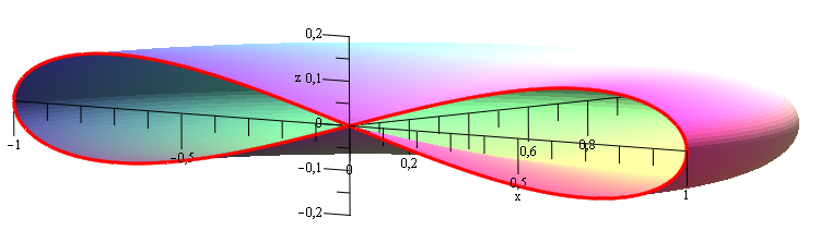
It is evident that the vertical axis \(Oz\) is ‘forbidden' — points \(p_i\) and \(p_j\) having different \(z\) coordinate define parallel planes \(\Pi _i\) and \(\Pi _j\). Consequently, the lsR -distance \(\mathbf {d}_{\mathrm
{lsR}}(O,(0,0,z))\) becomes infinite (as illustrated in Fig. 2). This contrasts with the standard sub-Riemannian ball in the Heisenberg group, which takes on an ‘apple' shape [6] , [7] . In contrast, the lsR -distance results in a pinched ball resembling a donut with an infinitely small hole.
The sub-Riemannian distance \(\mathbf {d}_{\mathrm {sR}}\) from the origin \(O\) to the point \((x,y,z)\) in the Heisenberg group \(\mathcal {H}\) is defined as follows [7] :
a) if \(z = 0\), then \(\mathbf {d}_{\mathrm {sR}}(O, (x,y,0)) =\sqrt {x^2+y^2}\),
b) if \(z\neq 0\) and \(x=y=0\), then \(\mathbf {d}_{\mathrm {sR}}(O,(0,0,z)) = \sqrt {2\pi |z|}\),
c) if \(z \neq 0\) and \(x^2+y^2>0\), then \(\mathbf {d}_{\mathrm {sR}}(O,(x,y,z)) =\frac {q}{\sin q}\sqrt {x^2+y^2}\),
where
\begin{equation}
\label {eq8} \frac {2q-\sin 2q}{4\sin ^2 q}=\frac {z}{x^2+y^2}.
\end{equation}
The Taylor expansion of ( 7 ) gives
\[ \mathbf {d}_{\mathrm {lsR}}(O,(x,y,z))=\sqrt {x^2+y^2}\big (1+\frac {1}{2}\frac {z^2}{(x^2+y^2)^2}(2+\sqrt {4+x^2+y^2})^2+ ...\big ). \]
In the general case c) of the sub-Riemannian distance, assuming that \(q\) is small enough, from ( 8 ) one gets
\[ q\sim \frac {3z}{x^2+y^2}. \]
Then
\[ \mathbf {d}_{\mathrm {sR}}(O,(x,y,z))=\sqrt {x^2+y^2}\big ( 1 + \frac {1}{2}\frac {3z^2}{(x^2+y^2)^2} + ...\big ). \]
The second term in this expansion can be interpreted as a sub-Riemannian correction to the 2-dimensional Euclidean distance function \(\sqrt {x^2+y^2}\). Notably, both corrections share a common multiplier of the form \(\frac {3z^2}{(x^2+y^2)^2}\), which is a
positive indication. It is possible to introduce an additional parameter \(\Lambda \) into the lsR -distance ( 7 ) that changes the weight of the
\((\rho (p_i^{\bot }, p_j^{\bot }))^2\) summand, namely
\[ \sqrt {x^2+y^2}\cdot \sqrt {1+\Lambda \frac {z^2}{(x^2+y^2)^2}(2+\sqrt {4+x^2+y^2})^2}. \]
As \(\Lambda \) approaches zero, the ball \(B(O, 1)\) becomes thicker; conversely, as \(\Lambda \rightarrow \infty \), it flattens out — transforming from a donut to a pancake: \(B(O,1)\rightarrow D_1\). It is crucial to note that if the lsR -ball \(B(O,1)\) were merely a 2-dimensional disc \(D_1\), then the distance between almost any pair of random points would be infinite.
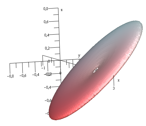
If the center of the ball shifts from the origin to the point \(p_i\), the ball bends in such a way that its central plane of symmetry coincides with the plane \(\Pi _i\) of admissible directions at \(p_i\) (Fig.3).
Consider the cubic domain \(\Omega =[-1,1]^3\subset \mathcal {H}\) with a set \(D=\{p_i\in \Omega |i=1,\ldots , N \}\) of \(N\) points. These points can form either a regular lattice or they can be randomly and uniformly distributed in \(\Omega \). We will
consider the scenario with random points. Calculate all distances \(\mathbf {d}_{\mathrm {lsR}}(p_i,p_j)\) using ( 6 ) and consider the weighted spatial graph \(\Gamma
_r\) with vertices \(p_i\) and edges \(v_{ij}\) of weight \(\mathbf {d}_{\mathrm {lsR}}(p_i,p_j)\leq r\), it means that vertices \(p_i \in D\) and \(p_j\) are connected by the edge \(v_{ij}\) in the graph \(\Gamma _r\) if and only if the local sub-Riemannian
distance \(\mathbf {d}_{\mathrm {lsR}}(p_i,p_j)\) between them is smaller than a fixed value \(r\).
The graph \(\Gamma _r\) serves as a discrete model for the Heisenberg group. When the parameter \(r\) is too small, most vertices in \(\Gamma _r\) tend to be disjoint. Conversely, if \(r\) is excessively large, nearly all pairs of points \((p_i,p_j)\) will be connected by
an edge. The critical threshold value \(r^{\ast }\) is influenced by both the number of vertices \(N\) and the domain \(\Omega \). Here, \(r^{\ast }\) refers to the specific value of \(r\) such that for any \(r > r^{\ast }\), the graph \(\Gamma _r\) becomes
connected for an average distribution of the points \(p_i\).
Next we perform a number of numerical experiments demonstrating that the presented discrete model possesses features specific for the sub-Riemannian Heisenberg group. Firstly, using the standard Dijkstra algorithm [8] for finding shortest paths in a graph, one can find the shortest path in \(\Gamma _r\). The shortest path is a broken line with vertices at the points
\(p_1,p_{i_1},\ldots ,p_{i_k},p_2\), thus the discrete sub-Riemannian (dsR) distance between \(p_1\) and \(p_2\) in \(\Gamma _r\) is
\begin{equation}
\label {eq9} \mathbf {d}_{\mathrm {dsR}}(p_1,p_2)= \mathbf {d}_{\mathrm {lsR}}(p_1,p_{i_1})+\mathbf {d}_{\mathrm {lsR}}(p_{i_1},p_{i_2})+\ldots +\mathbf {d}_{\mathrm {lsR}}(p_{i_k},p_2).
\end{equation}
Numerical calculations show that the shortest path between \(p_1=(0,0,0)\) and \(p_2=(0,0,z_2)\) has a form of a single-wind helix (Fig.4) — a typical form for the Heisenberg geodesics [7] , [9] :
\begin{equation}
\label {eq10} \begin{cases} x(t)&=(\sin (\theta _0+h_3t)-\sin \theta _0)/h_3,\\ y(t)&=(\cos \theta _0-\cos ( \theta _0+h_3t))/h_3, \\ z(t)&=(h_3t-\sin h_3t)/h^2_3. \end {cases}
\end{equation}
Next we compare the distance \(\mathbf {d}_{\mathrm {dsR}}\) between points as the vertices of the graph \(\Gamma _r\) and the sub-Riemannian distance \(\mathbf {d}_{\mathrm {sR}}\) in \(\mathcal {H}\). We will consider two situations: horizontal and vertical.
In the horizontal case, when \(p_1=(0,0,0)\) and \(p_2=(x_2,y_2,0)\), the geodesic in \(\mathcal {H}\) is a straight horizontal interval \([p_1,p_2]\) in the plane \(\mathrm {Oxy}\). The vertical situation is when \(p_1=(0,0,0)\) and \(p_2=(0,0,z_2)\) and the
geodesic is a helix (10) with non-constant slope. In accordance with a) the sub-Riemannian distance in the horizontal case coincides with the Euclidean length \(\mathbf {d}_{sR}((0,0,0),(x_2,y_2,0))= \sqrt {x_2^2+y_2^2}\).
If the number of vertices \(N\) is small, the graph \(\Gamma _{r}\) can be disconnected, in which case the distance between disconnected vertices is equal to infinity. In Table
1 the value 0.8955 is the averaged distance of \(\mathbf {d}_{\mathrm {dsR}}(p_1,p_2)\) calculated for 10 numerical experiments with 4000 random vertices each. As \(N\) increases, the dispersion of \(\mathbf {d}_{dsR}(p_1,p_2)\) decreases
and its value gets closer to the value of \(\mathbf {d}_{sR}(p_1,p_2)\). The convergence of the distances in the vertical case is shown in Table 2 .
From Tables 1 and 2 one can see that, as \(N\) increases, the discrete sub-Riemannian distance gets closer to the standard sub-Riemannian distance in \(\mathcal {H}\), but with different rates in the horizontal and vertical cases. A more detailed discussion on these
results will be provided in the next section.
The last feature of geodesics in \(\mathcal {H}\) that is going to be checked for \(\Gamma _r\) is the fact that the coordinate \(z(t)\) of the geodesic that starts at \(O\) is proportional to the sectional area of the projection \((x(t),y(t))\) onto the \(Oxy\) plane. For
the considered discrete model this projection is a polygon, see the upper right picture in Fig.4 The numerical experiment is the following:
1. Pick \(M\) test vertices \(p\) in \(\Gamma _r\), whose third coordinate is \(z(p)\);
2. Find the shortest path from \(O\) to \(p\);
3. Calculate the polygon area \(A(p)\) of the projected path.
For the Heisenberg group \(z(p)\) and \(A(p)\) are the same values, and, for example, the Dido's problem can easily be reformulated as a problem of finding geodesics [7] . The results for \(\Gamma _{\frac {1}{2}}\) with \(N=3000\) random vertices and with \(M=200\) test vertices are presented in the Fig. 5. As the coordinate \(z(p)\) is uniformly distributed in
\([-1,1]\), the dots with coordinates \((z(p),A(p))\) on Fig. 5 lie quite close to the plot of \(|z(p)|\).
First let us recall briefly what tortuosity is. Consider a domain \(\Omega ' \subset \mathbb {R}^3\) modeling a piece of porous media, such that there is a connected subset \(P\subset \Omega '\) modeling the system of
the media pores. Next, \(\Omega ' \setminus P\) simulates solid material. One can consider two arbitrary points \(A,B \in P\) and the shortest path \(\gamma (t),~ t\in [0,1]\) connecting \(A\) and \(B\) that fully lies in the system of pores \(P\): \(\forall
t\in [0,1] ~~ \gamma (t)\in P\). The ratio of the length of \(\gamma \) and the standard Euclidean distance between \(A\) and \(B\)
\[ \frac {\int \limits _0^1 |\dot {\gamma }(t)| dt }{\mathrm {dist}_{Eucl}(A,B)} \]
called the tortuosity \(\tau \) of the path \(\gamma (t)\). If the media is homogeneous and isotropic and if \(\mathrm {dist}_{Eucl}(A,B)\) is sufficiently large, the tortuosity will be close to a limit value: it is greater than \(1\) and
measures the level of entanglement of the system of pores. If the media is anisotropic then \(\tau (A,B)\) will depend on the direction \(\overrightarrow {AB}\).
Secondly, one can study the tortuosity of the Delaunay triangulation of uniformly distributed points [10] . It turns out
that the ratio between the length \(l_{triang}(A,B)\) of the shortest broken line connecting two points via edges of the triangulation and the Euclidean distance,
\[ \frac {l_{triang}(A,B) }{\mathrm {dist}_{Eucl}(A,B)}, \]
converges from above to a fixed value \(\tau _{Dln}\approx 1.05\) for a two-dimensional domain and \(\tau _{Dln}\approx 1.09\) for a three-dimensional domain.
Next we come back to a domain \(\Omega \) with the standard sub-Riemannian metric \(\mathbf {d}_{\mathrm {sR}}\) and the spatial graph \(\Gamma _r\) in \(\Omega \) with vertices \(p_i \in D\) and metric \(\mathbf {d}_{\mathrm {dsR}}\). The following ratio
\begin{equation}
\label {eq11} \tau (A,B)= \frac {\mathbf {d}_{\mathrm {dsR}}(A,B)}{\mathbf {d}_{\mathrm {sR}}(A,B)}
\end{equation}
Let us consider again two points \(A=p_1\) and \(B=p_2\) from the previous section. From Table 1, when both points lie in the horizontal plane \(\{z=0\}\) and the sub-Riemannian geodesic is a straight line, the tortuosity (11) gets close to \(\tau _{Dln}\) in the
three-dimensional case of the Delaunay tortuosity.
In the case of helicoidal geodesic, the difference between the sub-Riemannian and discrete sub-Riemannian distances becomes more evident:
Considering this ‘anisotropic' behaviour of \(\tau (A,B)\) we formulate the following
Conjecture on the limit tortuosity. Consider a cubic domain \(\Omega \subset \mathcal {H}\) with the sub-Riemannian distance \(\mathbf {d}_{\mathrm {sR}}\) and the corresponding spatial graph \(\Gamma _r\) with \(N\)
uniformly distributed vertices \(D\) and the discrete sub-Riemannian distance \(\mathbf {d}_{\mathrm {dsR}}\). Fix two points \(A=(0,0,0)\in D\) and \(B=(\cos \varphi , 0, \sin \varphi )\in D\). As \(N\rightarrow \infty \) one can choose a parameter of the
graph \(\Gamma _r\) with the asymptotic such that the tortuosity \(\tau (A,B)\) converges to a limit tortuosity \(\tilde {\tau }=\tilde {\tau }(\varphi )\) depending only on the coordinate \(\varphi \) of \(B\) for almost all positions of vertices in \(D\). The limit tortuosity should be bounded
\[ 1<\tilde {\tau }< C ~~~~~~\forall \varphi \in [0,2\pi ]. \]
Due to the fact that all considered functions are random variables the convergence of the tortuosity in this conjecture should be almost sure convergence. Finding optimal bounds for the constants \(c\), \(d\) and \(C\) is another problem to consider. Also, the connection
between \(d\) and the dimension (topological or Hausdorf) of the Heisenberg group is not clear.
We will say that a broken line with vertices \(A=p_{i_1},p_{i_2}, \ldots , p_{i_k}=B\) is \(\varepsilon \)-close to a geodesic \(\gamma (t)\), \(t\in [t_0,t_1]\), connecting \(A\) and \(B\) if there is a cylindrical neighbourhood of \(\gamma (t)\)
\[ Cyl_{\varepsilon } =\bigcup \limits _{t\in [t_0,t_1]} \{\gamma (t) + v | \forall v\in \mathbb {R}^3, ~ |v|\leq \varepsilon \}, \]
containing all vertices \(p_i\) and all edges \([p_{i_j}, p_{i_j+1}]\) of the broken line.
Finally, we can formulate the approximation conjecture:
Approximation Conjecture. Consider a cubic domain \(\Omega \subset \mathcal {H}\) with the sub-Riemannian distance \(\mathbf {d}_{\mathrm {sR}}\), the orresponding spatial graph \(\Gamma _r\) with \(N\) uniformly
distributed vertices \(D\) and the discrete sub-Riemannian distance \(\mathbf {d}_{\mathrm {dsR}}\). Fix two points \(A=O\in D\) and arbitrary \(B\in D\) and a sub-Riemannian geodesic \(\gamma (t)\) connecting \(A=\gamma (t_0)\) and \(B=\gamma (t_1)\). For
any \(\epsilon \) there is number \(N\) of vertices and a parameter \(r\) satisfying (12) such that there is a shortest path \(A=p_{i_1},p_{i_2}, \ldots , p_{i_k}=B\) in the graph \(\Gamma _r\) which is \(\varepsilon \)-close to \(\gamma (t)\).
Note that if the point \(B\) lies on the \(Oz\) axis then there is no uniqueness of the sub-Riemannian geodesic connecting \(A=O\) and \(B\), it is defined up to rotation as it was mentioned earlier. In this case in the approximate conjecture one should choose an
appropriate geodesic. It seems to be clear how to prove that in a cylindric neighbourhood of the fixed geodesic there is a broken line with vertices and edges from \(\Gamma _r\). But how to prove that this broken line will be globally shortest path in \(\Gamma _r\)?
Here we presented a discrete model \(\Gamma _r\) of the Heisenberg group \(\mathcal {H}\) as a spatial graph with weighted edges. The weight of the edge is defined by the local sub-Riemannian distance \(\mathbf {d}_{lsR}\), generated by the non-integrable
Heisenberg distribution ( 1 ). The discrete sub-Riemannian distance \(\mathbf {d}_{dsR}\) is the length of a shortest path in \(\Gamma _r\). Numerical experiments give a
motivation to formulate an approximation conjecture stating that shortest paths in the graph \(\Gamma _r\) will be sufficiently close to the geodesics in \(\mathcal {H}\) if the number of vertices \(N\) is large enough and the parameter \(r\) is appropriately small.
The constructed model can be considered as a ‘triangulation of the sub-Riemannian Heisenberg group', but without triangles. The triangulation of a smooth two-dimensional surface embedded in \(\mathbb {R}^3\) is a collection of vertices, edges and triangles. In the
non-integrable case there is no surface, so there should be no triangles. It is natural to choose a spatial graph \(\Gamma _r\), consisting only of vertices and edges, as a model for non-integrable geometry.
We believe that the presented construction will be interesting both for specialists in discrete geometry and in sub-Riemannian geometry. The presented model can be useful for simulations of various processes in anisotropic medias, such as heat propagation, diffusion in
anisotropic porous materials, deformations of layered solids, etc.
[1] E. Malkovich. On discrete sub-Riemannian geometry. International Conference on Geometric Analysis, 2022, p.82.
[2] J.E. Marsden, M. West. Discrete mechanics and variational integrators. Acta Numerica, 2001, 357-514.
[3] A.A. Simoes, J.C. Marrero, D.M. de Diego. Exact discrete Lagrangian mechanics for nonholonomic mechanics. Numerische Mathematik, Vol. 151, p. 49-98, 2022.
[4] Yu.N. Fedorov, D.V. Zenkov. Discrete nonholonomic LL systems on Lie groups. Nonlinearity 18(2005), 2211-2241.
[5] P.Popescu, M. Popescu. On discrete geometry of non-holonomic spaces. Proceedings of The International Conference "Differential Geometry and Dynamical Systems" (DGDS-2014), 1-4 September 2014, Mangalia, ROMANIA, BSG PROCEEDINGS 22 (2015)
69-74.
[6] V.N. Berestovskii, I.A. Zubareva. Shapes of spheres of special nonholonomic left-invariant intrinsic metrics on some Lie groups. Siberian Math. J.42(2001), no.4, 613–628.
[7] Yu. Sachkov. Introduction to Geometric Control. Springer Nature, 2022.
[8] E.W. Dijkstra. A note on two problems in connexion with graphs. Numerische Mathematik. (1959), 1: 269–271.
[9] V.N. Berestovskii. Geodesics of nonholonomic left-invariant intrinsic metrics on the Heisenberg group and isoperimetric curves on the Minkowski plane. Siberian Math. J., 35:1 (1994), 1–8.
[10] A.A. Bystrov, E.G. Malkovich. Tortuosity of Delaunay Triangulations and Statistics of Shortest Paths. Experimental Mathematics, 2024, October, 1–7. doi:10.1080/10586458.2024.2410189.
1. Introduction
2. Local sub-Riemannian Distance
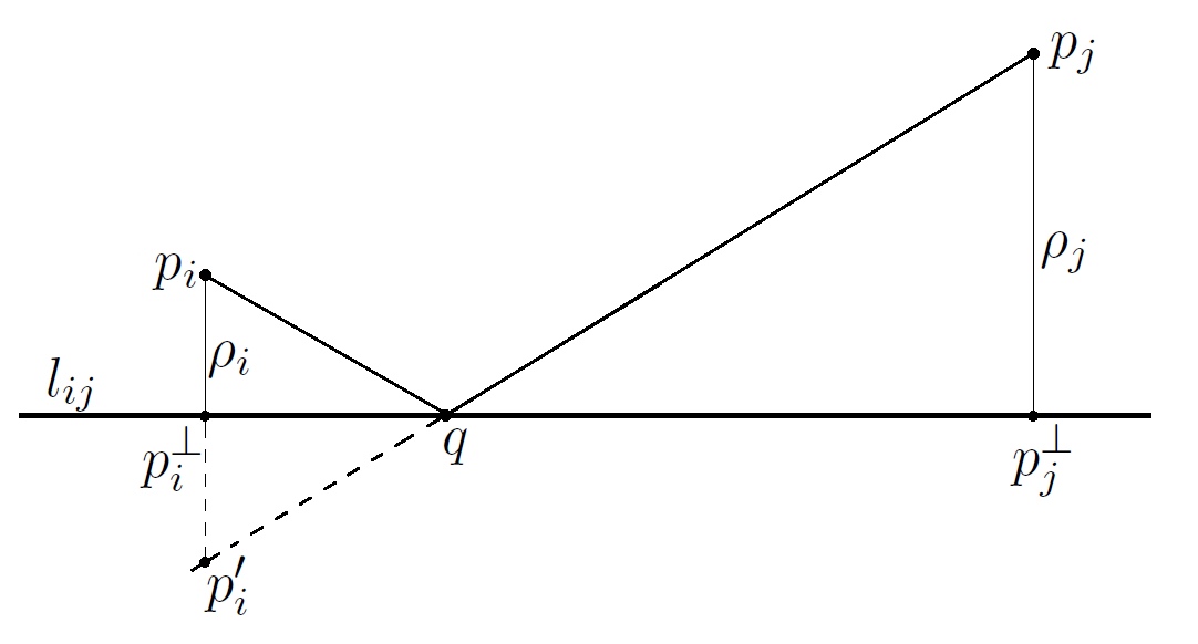
Figure 1. The local sub-Riemannian distance \(\mathbf {d}_{\mathrm {lsR}}(p_i,p_j)\) and Heron's problem.
3. A spatial graph and a discrete sub-Riemannian distance
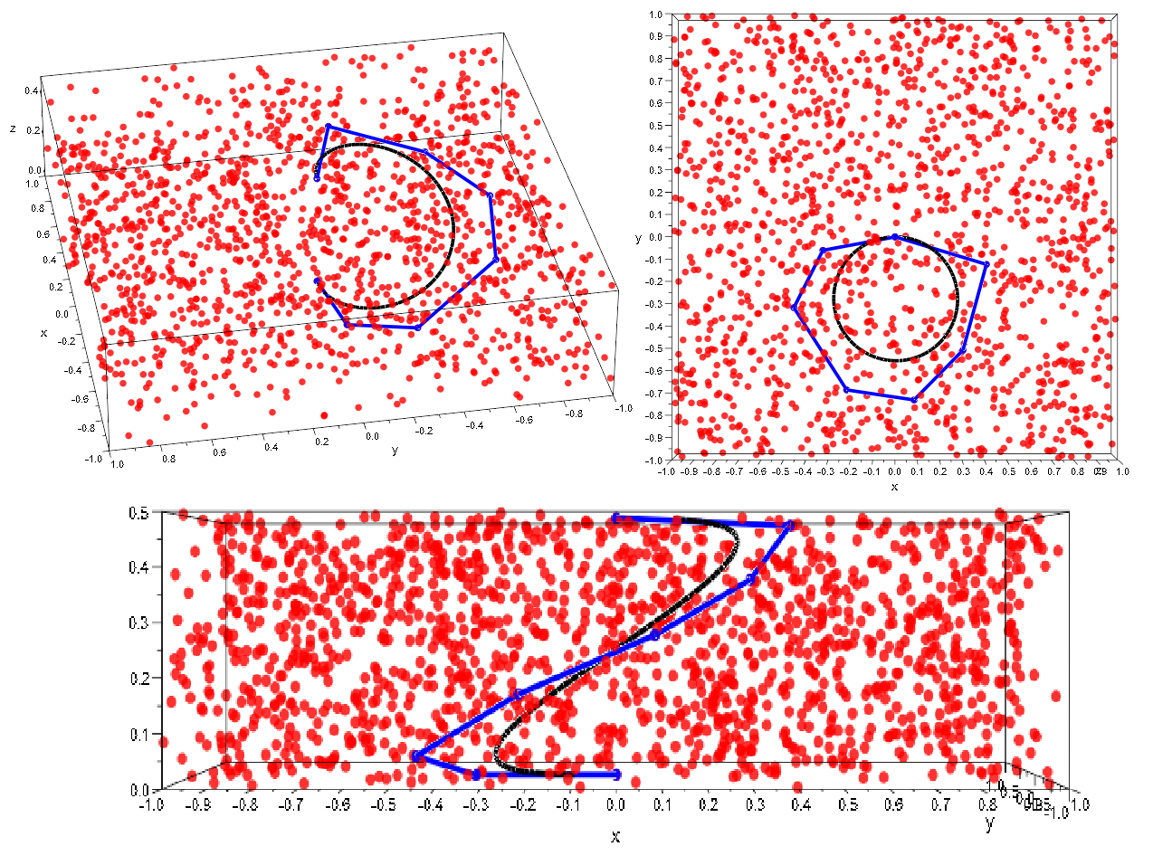
Figure 4. Sub-Riemannian geodesic (black, (10)) and typical shortest path (blue) in the graph \(\Gamma _{\frac {1}{2}}\) with \(N=1500\) vertices connecting points \((0,0,0)\) and
\((0,0,\frac {1}{2})\), various projections.
\(N=1000\)
\(N=2000\)
\(N=4000\)
\(N=6000\)
\(\mathbf {d}_{sR}(p_1,p_2)\)
\(x_2=y_2=\frac {1}{2}\)
1.8628
0.8971
0.8655
0.7752
\(\frac {\sqrt {2}}{2}\approx 0.7071\)
\(x_2=y_2=1\)
\(\infty \)
1.9839
1.7267
1.5965
\(\sqrt {2}\approx 1.4142\)
Table 1. Mean distance \(\mathbf {d}_{\mathrm {dsR}}((0,0,0),(x_2,y_2,0))\) for different \(N\) and sub-Riemannian distance, horizontal case.
\(N=1000\)
\(N=2000\)
\(N=4000\)
\(N=6000\)
\(\mathbf {d}_{sR}(p_1,p_2)\)
\(z_2=\frac {1}{9}\)
1.717
1.3617
1.2929
1.2702
\(\frac {\sqrt {2\pi }}{3}\approx 0.8355\)
\(z_2=\frac {4}{9}\)
3.2894
2.8339
2.5877
2.5209
\(\frac {2\sqrt {2\pi }}{3}\approx 1.671\)
Table 2. Mean distance \(\mathbf {d}_{\mathrm {dsR}}((0,0,0),(0,0,z_2))\) for different \(N\) and the sub-Riemannian distance, vertical case.
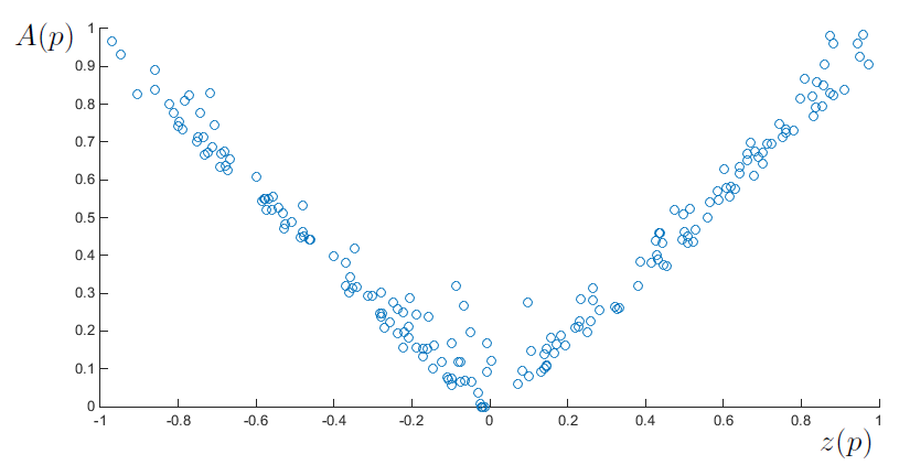
Figure 5. The coordinate \(z(p)\) and the area \(A(p)\) of the projected polygon for \(M=200\) test vertices in \(\Gamma _{\frac {1}{2}}\).
4. Tortuosity
\(N=1000\)
\(N=2000\)
\(N=4000\)
\(N=6000\)
\(x_2=y_2=\frac {1}{2}\)
2.6344
1.2687
1.2240
1.0963
\(x_2=y_2=1\)
\(\infty \)
1.4028
1.2210
1.1289
Table 3. The tortuosity \(\tau ((0,0,0),(x_2,y_2,0))\) for different \(N\), horizontal case.
\(N=1000\)
\(N=2000\)
\(N=4000\)
\(N=6000\)
\(z_2=\frac {1}{9}\)
2.0551
1.6298
1.5475
1.5203
\(z_2=\frac {4}{9}\)
1.9685
1.6959
1.5486
1.5086
Table 4. The tortuosity \(\tau ((0,0,0),(0,0,z_2))\) for different \(N\), vertical case.
5. Conclusion.
References
MMM