Arnold Mathematical Journal
Volume 12, Issue ?, 2026

Research Contribution DOI:10.56994/ARMJ.012.00?.00?
Received: 20 Sep 2025; Accepted: 22 Jun 2025

Symmetric cubic polynomials

Alexander Blokh , Lex Oversteegen , Nikita Selinger , Vladlen Timorin and Sandeep Chowdary Vejandla Department of Mathematics
University of Alabama at Birmingham
Birmingham, AL 35294 Faculty of Mathematics
National Research University Higher School of Economics
6 Usacheva str., Moscow, Russia, 119048 ablokh@math.uab.edu overstee@uab.edu selinger@uab.edu vsc4u@uab.edu vtimorin@hse.ru

(Date: September 20, 2024; revised May 23, 2025)

Abstact.

Key words and phrases:

Complex dynamics; laminations; Mandelbrot set; Julia set

2010 Mathematics Subject Classification:

Primary 37F20; Secondary 37F10, 37F50

The first named author was partially supported by NSF grant DMS-2349942. The second named author was partially supported by NSF grant DMS–1807558. The work of the fourth named author was supported by the HSE University Basic Research Program.

1 Introduction

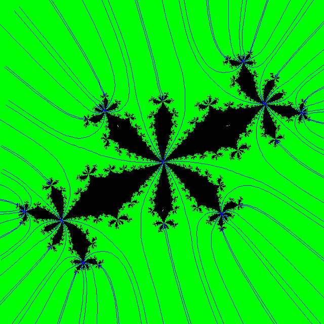
A central problem of Complex Dynamics is to describe parameter spaces of holomorphic maps. Investigating the deceptively simple quadratic family $f_{c}(z)=z^{2}+c$ led to an explosion of activity in the field. Aided by computer graphics capabilities, mathematicians made many interesting discoveries concerning the connectedness locus of the quadratic family, the celebrated Mandelbrot set $\mathcal{M}_{2}$ .

One of the first such discoveries, made by Douady and Hubbard [15], was that $\mathcal{M}_{2}$ is connected. Then the combinatorial description of the structure of the Mandelbrot set was largely carried out in the language of laminations introduced by Thurston [41] (see Section 3 and [41] or [6] for precise definitions and other details). Douady constructed a topological pinched disk model of $\mathcal{M}_{2}$ ; Thurston made this model more explicit and described it in terms of laminations. If $\mathcal{M}_{2}$ is locally connected (which is still an open question), then it is homeomorphic to its model. The local connectivity of the Mandelbrot set is one of the most important long standing conjectures in the field; if true, it will imply the density of hyperbolicity property of the quadratic family.

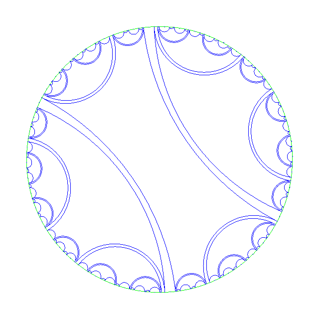
The above describes the quadratic version of what one can call the Douady–Hubbard–Thurston program, i.e. a two step approach to studying some complex one-dimensional parameter space of polynomials that we now fix. Similar to the quadratic family, its most interesting part is the connectedness locus, i.e., the locus of all polynomials in the space with connected Julia sets (in the quadratic case, this is the Mandelbrot set). One needs to prove that the connectedness locus is connected itself. Then two steps are made. On the first step one describes the laminations of the polynomials from the parameter space in question producing in the end the corresponding space of laminations, most likely described itself by a certain parameter lamination (like, e.g., Thurston’s QML lamination [41]). On the second step one constructs a monotone map from the connectedness locus of interest to the quotient space of the closed unit disk under the parameter lamination. This quotient space can be viewed as a model for the connectedness locus.

The Douady–Hubbard–Thurston program has been implemented for quadratic polynomials, and then for unicritical polynomials $z^{d}+c$ of any degree $d$ , cf. [1, 22, 38, 39], where $c$ is the parameter.

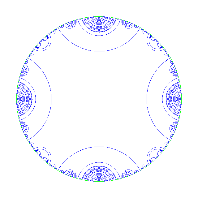
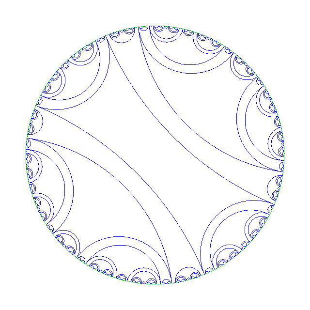
We initiated this program for the space $\mathcal{SCP}$ of symmetric cubic polynomials $p_{c}(z)=z^{3}-3c^{2}z$ with marked critical point $c$ in papers [8, 9] that serve as a prequel to the present article. Namely, in [8] we investigated the space of symmetric cubic laminations and constructed the associated parameter lamination called the cubic symmetric comajor lamination $C_{s}CL$ (see Section 3). In [9] we proved an analog of Lavaurs algorithm for this lamination. Now, let $\mathcal{M}^{sy}_{3}$ be the connectedness locus of $\mathcal{SCP}$ . The aim of the present article is to complete the program for the space $\mathcal{SCP}$ and prove the following theorem.

Main Theorem.

The set $\mathcal{M}^{sy}_{3}$ is a full continuum. There exists a monotone continuous surjective map $\pi:\mathcal{M}^{sy}_{3}\to\overline{\mathbb{D}}/C_{s}CL$ . If $\mathcal{M}^{sy}_{3}$ is locally connected, then $\pi$ is a homeomorphism.

We are not aware of any other articles in which the Douady–Hubbard–Thurston program is fully implemented for non-unicritical polynomials. We did recently learn of a manuscript by Xavier Buff [12] in which he studies the parameter space of symmetric polynomials of the form $P_{\lambda,d}(z)=\lambda z+z^{d}$ and shows that the connectedness locus $M_{d}$ contains the unit disk $\mathbb{D}$ and that every component of $M_{d}\setminus\overline{\mathbb{D}}$ is homeomorphic to a limb of the Mandelbrot set.

Acknowledgments.

2 Notation and preliminaries

We assume knowledge of basic facts and concepts of complex dynamics. We also use standard notation (such as $J(P)$ for the Julia set of a polynomial $P$ , etc).

Consider the space $\mathcal{SCP}$ of symmetric cubic polynomials $p_{c}(z)=z^{3}-3c^{2}z$ with marked critical point $c$ , or, more formally, the space of pairs $(p_{c},c)$ , which, in turn, is uniquely parameterized by the values of $c$ . Since $p_{c}=p_{-c}$ , every polynomial (except for $p_{0}(z)=z^{3}$ ) shows in $\mathcal{SCP}$ twice. Thus, $\mathcal{SCP}$ is a (branched) two-to-one cover of the moduli space of all odd cubic polynomials, where the moduli space means the quotient space with respect to complex linear conjugacy. The critical points of $p_{c}$ are $c$ and $-c$ , the corresponding critical values are $-2c^{3}$ and $2c^{3}$ . The marked cocritical point of $p_{c}$ , i.e., the other preimage of $-2c^{3}=p_{c}(c)$ , is $-2c$ . Subsets $A$ and $B$ of the plane are said to be mutually symmetric if $B=-A$ . If $A=-A$ we call a set $A$ symmetric. Since $p_{c}$ is odd, the Julia set $J(p_{c}),$ the filled Julia set $K(p_{c})$ , and their complements are symmetric. Observe that $p_{c}(0)=0$ and $p^{\prime}_{c}(z)=p^{\prime}_{c}(-z)=3z^{2}-3c^{2}$ .

Let $\mathcal{M}^{sy}_{3}$ be the connectedness locus of $\mathcal{SCP}$ , i.e., the set of all $c$ for which the Julia set of $p_{c}$ is connected. It is known that the Julia set of $p_{c}$ is connected if and only if all forward orbits of critical points of $p_{c}$ are bounded. Since $p_{c}$ has mutually symmetric critical orbits, we conclude that $c\in\mathcal{M}^{sy}_{3}$ if and only if the orbit of $c$ or, equivalently of $-2c$ or $2c$ , is bounded.

For any $r>0$ set $\mathbb{D}_{r}=\{z\in\mathbb{C}\,|\,|z|<r\}$ , and write $\mathbb{D}$ for $\mathbb{D}_{1}$ . Let $\mathbb{S}^{1}$ be the unit circle. For a set $A\subset\mathbb{C}$ , let $\overline{A}$ be its closure and $\partial A$ be its boundary. We use the terms periodic orbit and cycle interchangeably. External rays to the Julia set of a polynomial $P$ are denoted $R_{P}(\theta)$ where $\theta$ is the argument of the ray (if there is no ambiguity we may omit the polynomial from our notation; also, we write $R_{c}(\theta)$ instead of $R_{p_{c}}(\theta)$ ).

Let $X$ , $Y$ be topological spaces and $f:X\rightarrow Y$ be continuous. Then $f$ is said to be monotone if $f^{-1}(y)$ is connected for each $y\in Y$ . It is known that if $f$ is monotone and $X$ is a continuum then $f^{-1}(Z)$ is connected for every connected $Z\subset f(X)$ .

Refer to caption — Figure 1. The parameter space of symmetric cubic polynomials $\mathcal{SCP}$ on the left and the Symmetric Cubic Comajor Lamination $C_{s}CL$ on the right.

3 Symmetric cubic laminations

Invariant laminations were introduced in [41]; they play a major role in polynomial dynamics. The preceding papers [8, 9] of this series contain an overview, based on [41] and [6]. Here we follow [8] and [9] (see Section 2 of [8] for a detailed discussion).

If a monic polynomial $P$ has a locally connected Julia set $J(P)$ , then $P|_{J(P)}$ is topologically conjugate to a suitable quotient of the $d$ -tupling map $\sigma_{d}:\mathbb{S}^{1}\to\mathbb{S}^{1}$ (where $\sigma_{d}(z)=z^{d}$ if $\mathbb{S}^{1}$ is viewed as the unit circle in $\mathbb{C}$ and as $\sigma_{d}(\theta)=d\theta$ if $\mathbb{S}^{1}$ is identified with $\mathbb{R}/\mathbb{Z}$ ). The quotient is with respect to an equivalence relation $\sim_{P}$ ; the leaves of the corresponding lamination $\mathcal{L}_{P}$ are by definition the edges of the convex hulls of all $\sim_{P}$ -classes.

A chord of $\overline{\mathbb{D}}$ with endpoints $a, b$ is denoted by $\overline{ab}$ ; it is critical if $\sigma_{d}(a)=\sigma_{d}(b)$ while $a\neq b$ . A lamination is normally denoted by $\mathcal{L}$ while the union of all its leaves and $\mathbb{S}^{1}$ by $\mathcal{L}^{*}$ . For $G\subset\overline{\mathbb{D}}$ , denote $G\cap\mathbb{S}^{1}$ by $\mathcal{V}(G)$ and call the elements of $\mathcal{V}(G)$ vertices of $G$ . Call $G$ a gap of a lamination $\mathcal{L}$ if it is the closure of a component of $\mathbb{D}\setminus\mathcal{L}^{\ast}$ . A gap $G$ is said to be critical if its image is not a gap or the degree of $\sigma_{d}|_{\partial G}$ is greater than 1. A critical set is a critical leaf or a critical gap. If $G$ is a leaf or a gap of $\mathcal{L}$ , then $G$ coincides with the convex hull of $\mathcal{V}(G)$ . A gap $G$ is called infinite (finite) if and only if $\mathcal{V}(G)$ is infinite (finite).

Let $\mathcal{L}$ be a lamination. The equivalence relation $\sim_{\mathcal{L}}$ induced by $\mathcal{L}$ is defined by declaring that $x\sim_{\mathcal{L}}y$ if and only if there exists a finite concatenation of leaves of $\mathcal{L}$ joining $x$ to $y$ . A lamination $\mathcal{L}$ is called a q-lamination if the convex hulls of $\sim_{\mathcal{L}}$ -classes are precisely finite gaps or leaves of $\mathcal{L}$ . Two distinct chords are called ( $\sigma_{d}$ -)siblings if they have the same $\sigma_{d}$ -image.

3.1 Symmetric laminations

Let $\tau$ be the rotation of $\overline{\mathbb{D}}$ (or of $\mathbb{S}^{1}$ ) by $180^{\degree}$ around its center $\mathcal{O}$ . Also, given a map $f:X\to X$ we call $x\in X$ preperiodic of preperiod $k>0$ or $k$ -preperiodic if $f^{k}(x)$ is $f$ -periodic while $f^{k-1}(x)$ is not periodic.

Definition 3.1 (Symmetric laminations).

A $\sigma_{3}$ -invariant lamination $\mathcal{L}$ is called a symmetric (cubic) lamination if $\ell\in\mathcal{L}$ implies $\tau(\ell)\in\mathcal{L}$ .

Definition 3.2 (length and majors).

Given a non-diameter chord $\ell$ in $\overline{\mathbb{D}}$ , define the arc $h(\ell)$ as the shortest arc of $\mathbb{S}^{1}$ joining the endpoints of $\ell$ . If $\ell^{\prime}$ and $\ell^{\prime\prime}$ are chords such that $h(\ell^{\prime})\subset h(\ell^{\prime\prime})$ , then we say that $\ell^{\prime}$ is under $\ell^{\prime\prime}$ . Define the length $|\ell|$ of $\ell$ as the length of $h(\ell)$ divided by $2\pi$ in the case when $\ell$ is not a diameter; if $\ell$ is a diameter, set $|\ell|=\frac{1}{2}$ . Given a symmetric lamination $\mathcal{L}$ , call a leaf $M$ a major of $\mathcal{L}$ if there are no leaves of $\mathcal{L}$ closer in length to $\frac{1}{3}$ than $M$ .

Let $\Gamma:[0,\frac{1}{2}]\to[0,\frac{1}{2}]$ be a piecewise linear function with slope $\pm 3$ defined as $\Gamma(x)=3x$ if $0\leq x\leq\frac{1}{6}$ and as $\Gamma(x)=|3x-1|$ if $\frac{1}{6}\leq x\leq\frac{1}{2}$ . Then $|\sigma_{3}(\ell)|=\Gamma(|\ell|)$ . Simple analysis of the dynamics of $\Gamma$ shows that for any leaf $\ell$ an eventual image of $\ell$ has length $0$ , or length $\frac{1}{2}$ , or length which is between $\frac{1}{4}$ and $\frac{5}{12}$ .

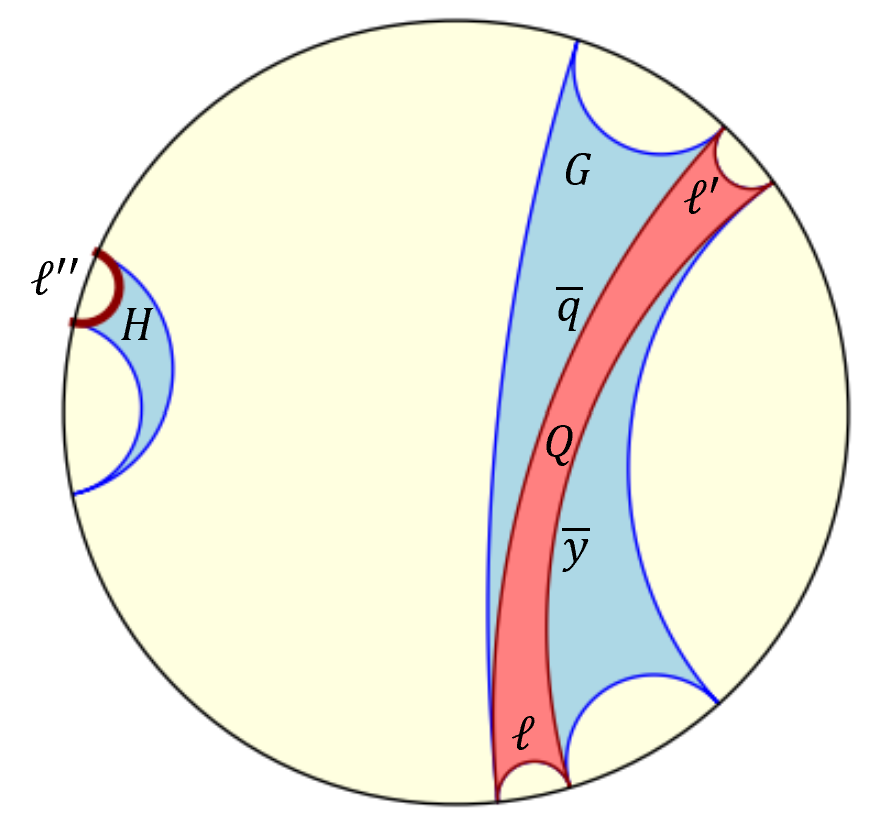
Suppose that $\frac{1}{4}\leq|\ell|\leq\frac{5}{12}$ . Then there exists a sibling chord $\ell^{\prime}$ of $\ell$ such that the strip $S$ of $\overline{\mathbb{D}}$ between $\ell$ and $\ell^{\prime}$ has two circle arcs on its boundary, each at most $\frac{1}{6}$ long. We also consider chords $\tau(\ell)$ and $\tau(\ell^{\prime})$ as well as the $\overline{\mathbb{D}}$ -strip $\tau(S)$ between them. The union $S\cup\tau(S)$ , denoted $\mathrm{SH}(\ell)$ , is called the short strips set of $\ell$ .

If a major $M$ of a symmetric lamination $\mathcal{L}$ is critical, there is a unique point $x\in\mathbb{S}^{1}$ that is not an endpoint of $M$ with the same $\sigma_{3}$ -image as $M$ . This point $x$ is called a comajor (of $\mathcal{L}$ ). If $M$ is not critical, then a leaf $M^{\prime}$ (similar to $\ell^{\prime}$ from the above) and leaves $\tau(M)$ and $\tau(M^{\prime})$ are also majors of $\mathcal{L}$ . We set $\mathrm{SH}(\mathcal{L})=\mathrm{SH}(M)$ in this case and call this set the short strips set of $\mathcal{L}$ . Let us stress again that $\mathrm{SH}(\mathcal{L})$ is formed by two strips and that $\mathrm{SH}(M)=\mathrm{SH}(\tau(M))$ . The third sibling $\overline{c}$ of $M$ that is disjoint from $M\cup M^{\prime}$ , is of length at most $\frac{1}{6}$ . It is called a comajor (of $\mathcal{L}$ ). Similarly we define a cocritical set $\overline{\mathrm{co}}(U)$ of a critical set $U$ as the gap, or the leaf, or the point disjoint from $U$ but with the same image as $U$ .

Because of the symmetry, comajors, majors, etc., come in pairs. A pair of comajors $\overline{c},\tau(\overline{c})$ of a symmetric lamination $\mathcal{L}$ is called a symmetric comajor pair. It is degenerate if its elements are points and non-degenerate otherwise. For a symmetric lamination $\mathcal{L}$ we often assume that one of its majors is marked; we denote this major by $M_{\mathcal{L}}$ and the corresponding comajor by $\overline{\mathrm{co}}_{\mathcal{L}}$ . Observe that if $\mathcal{L}_{1}$ and $\mathcal{L}_{2}$ are symmetric laminations such that $\mathrm{SH}(\mathcal{L}_{1})\subset\mathrm{SH}(\mathcal{L}_{2})$ (e.g., if $\mathcal{L}_{2}\subset\mathcal{L}_{1}$ ) then the comajors of $\mathcal{L}_{1}$ are located under the comajors of $\mathcal{L}_{2}$ .

Lemma 3.3 ([8]).

Let $\ell$ be a leaf of a symmetric lamination $\mathcal{L}$ with $|\ell|\geq\frac{1}{4}$ . If $n>0$ is the least such that $\sigma_{3}^{n}(\ell)\subset\mathrm{SH}(\ell)$ , then the leaf $\sigma_{3}^{n}(\ell)$ non-strictly separates (in $\overline{\mathbb{D}}$ ) either $\ell$ from $\ell^{\prime},$ or $\tau(\ell)$ from $\tau(\ell^{\prime})$ . Thus, either $\sigma_{3}^{n}(\ell)$ equals one of the leaves $\ell,\ell^{\prime},\tau(\ell),\tau(\ell^{\prime}),$ or it is closer to $\frac{1}{3}$ in length than $\ell$ . In particular, forward images of majors/comajors of $\mathcal{L}$ never enter the open circle arcs on the boundary of the set $\mathrm{SH}(\mathcal{L})$ .

Lemma 3.3 motivates the next definition.

Definition 3.4 (Legal pairs).

If a symmetric pair $\{\overline{c},\tau(\overline{c})\}$ is either degenerate or satisfies the following conditions:

(a)

no two iterated forward images of $\overline{c},\tau(\overline{c})$ cross, and
(b)

no forward image of $\overline{c}$ crosses the interior of $\mathrm{SH}(M_{\overline{c}})$ ,

then $\{\overline{c},\tau(\overline{c})\}$ is said to be a legal pair.

Lemma 3.5 ([8]).

A legal pair $\{c,\tau(c)\}$ is the comajor pair of the symmetric lamination $\mathcal{L}(c)$ . A symmetric pair $\{c,\tau(c)\}$ is a comajor pair if and only if it is legal.

A symmetric lamination with an infinite gap such that the map $\sigma_{3}$ on it is of degree greater than 1 is called a Fatou lamination.

Lemma 3.6 ([8]).

A symmetric lamination is Fatou if and only if it has a preperiodic comajor of preperiod 1.

Suppose that $\mathcal{L}$ is a symmetric q-lamination with two finite critical gaps each of which is preperiodic of preperiod at least two. Then $\mathcal{L}$ is called a symmetric Misiurewicz lamination. A symmetric Misiurewicz lamination has a well defined pair of comajors. Suppose that the critical $\sim_{\mathcal{L}}$ -classes are gaps $G$ and $\tau(G)$ with at least $6$ vertices each. Then there are two cocritical gaps $H\neq G$ and $\tau(H)\neq\tau(G)$ of $\mathcal{L}$ such that $\sigma_{3}(H)=\sigma_{3}(G)$ and $\sigma_{3}(\tau(H))=\sigma_{3}(\tau(G))$ . One edge of $H$ and one edge of $\tau(H)$ are the comajors of $\mathcal{L}$ . Two majors of $\mathcal{L}$ are edges of $G$ that are siblings of the comajor edge of $H$ ; two other majors of $\mathcal{L}$ are edges of $\tau(G)$ that are siblings of the comajor edge of $\tau(H)$ . While other edges of $G$ and $\tau(G)$ are not siblings of the comajors, they can generate majors of other laminations that are finite tunings of $\mathcal{L}$ .

Indeed, suppose that $\ell$ and $\ell^{\prime}$ are two sibling edges of $G$ that are not majors. The convex hull of $\ell\cup\ell^{\prime}$ is a 4-gon $Q$ with two extra edges $\overline{y}$ and $\overline{q}$ not equal to $\ell$ or $\ell^{\prime}$ , see Fig. 2. Construct a new lamination $\mathcal{L}^{\prime}$ (not a $q$ -lamination) by inserting $\overline{y}$ and $\overline{q}$ in $G$ , pulling them back along the backward orbit of $G$ and then doing the same with $\tau(G)$ and its backward orbit. The majors of $\mathcal{L}^{\prime}$ are $\overline{y}$ and $\overline{q}$ and their $\tau$ -images. If $\ell^{\prime\prime}$ is a leaf of $\mathcal{L}$ which is not an edge of $G$ and is such that $\sigma_{3}(\ell^{\prime\prime})=\sigma_{3}(\ell)$ then $\ell^{\prime\prime}$ and $\tau(\ell^{\prime\prime})$ are the two comajors of $\mathcal{L}^{\prime}$ . Repeating this construction for all pairs of sibling edges of $G$ but the majors, we see that every edge of the cocritical gap $H$ or $\tau(H)$ is a comajor of a certain symmetric lamination which is a tuning of the original symmetric Misiurewicz lamination $\mathcal{L}$ . Call cocritical sets of Misiurewicz laminations Misiurewicz cocritical sets. By [8, Theorem 3.9], symmetric laminations have no wandering gaps. Therefore, the above is a full description of finite gaps formed by comajors. The cocritical gaps $H$ and $\tau(H)$ described above will be called Misiurewicz cocritical gaps; similarly, if a symmetric Misiurewicz q-lamination has critical 4-gons (not 6-gons or higher as was assumed above) we call its comajors Misiurewicz cocritical leaves.

Theorem 3.7 ([8, 9]).

The set of non-degenerate comajors of symmetric laminations is a q-lamination $\mathcal{L}$ invariant under $\tau$ that induces an equivalence relation $\sim_{\mathcal{L}}$ on $\mathbb{S}^{1}$ . For any non-degenerate comajor $\overline{c}$ (i.e., a leaf of $\mathcal{L}$ ) one of the following holds.

(1)

It is a two-sided limit leaf in $\mathcal{L}$ which is not eventually periodic.
(2)

It is a preperiodic leaf of $\mathcal{L}$ with preperiod at least $2$ which is either a two-sided limit leaf of $\mathcal{L}$ (in which case $\overline{c}$ is a Misiurewicz cocritical leaf), or an edge of a finite gap $H$ of $\mathcal{L}$ whose edges are limits of leaves in $\mathcal{L}$ disjoint from $H$ (in which case $H$ is a Misiurewicz cocritical gap).
(3)

It is a $1$ -preperiodic comajor of a Fatou lamination and is disjoint from all other leaves of $\mathcal{L}$ ; all such comajors $\overline{c}$ are dense in $\mathcal{L}$ and all 1-preperiodic angles are endpoint of such comajors.

Since comajors are leaves of q-laminations, their endpoints are either both not preperiodic, or both preperiodic with the same preperiod and the same period, or both periodic with the same period. All classes of $\sim_{\mathcal{L}}$ from Theorem 3.7 are finite. By Theorem 3.7, periodic points of $\mathbb{S}^{1}$ are degenerate comajors.

Definition 3.8.

The q-lamination from Theorem 3.7 is called the Cubic Symmetric Comajor Lamination and is denoted by $C_{s}CL$ . It induces an equivalence relation denoted $\sim_{sy}$ . The $\sim_{sy}$ -classes corresponding to symmetric Misiurewicz laminations are called Misiurewicz $\sim_{sy}$ -classes. Denote by $\mathcal{M}^{sy}_{3,comb}$ the quotient space $\overline{\mathbb{D}}/\sim_{sy}$ . Let $\mathfrak{pr}_{comb}:\overline{\mathbb{D}}\to\mathcal{M}^{sy}_{3,comb}$ be the corresponding quotient projection.

Theorem 3.7 verifies the density of hyperbolicity conjecture for $C_{s}CL$ .

Lemma 3.9.

Let $\mathcal{L}$ be a symmetric non-empty Fatou lamination. Then one of the following holds.

(B)

There is only one cycle $\mathcal{A}$ of Fatou gaps of $\mathcal{L}$ . It has even period $2m$ , and is $\tau$ -symmetric. The periodic majors $M$ and $\sigma_{3}^{m}(M)=\tau(M)$ of $\mathcal{L}$ are edges of critical gaps $U\in\mathcal{A}$ and $V=\sigma_{3}^{m}(U)=\tau(U)$ . Non-periodic majors of $\mathcal{L}$ are siblings of $M$ and $\tau(M)$ and edges of $U$ and $V$ , respectively. The remaining (i.e., not belonging to a major) $2m$ -periodic vertices $x, y$ of $U$ are such that $\sigma_{3}^{m}(x)=\tau(y)$ while $\sigma_{3}^{m}(y)=\tau(x)$ .
(D)

There are exactly two cycles of Fatou gaps of the same period, interchanged by $\tau$ . Critical gaps $U$ , $V=\tau(U)$ belong to different cycles. The periodic majors $M$ and $\tau(M)$ of $\mathcal{L}$ are edges of $U$ and $V$ , respectively. Non-periodic majors are siblings of $M$ and $\tau(M)$ and edges of $U$ and $V$ , respectively.

In either case all edges of infinite gaps are eventually mapped to periodic majors. The only periodic orbit of edges of a Fatou gap of $\mathcal{L}$ is the orbit of a major of $\mathcal{L}$ and it has the same period as the Fatou gap.

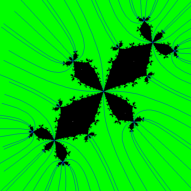
Lemma 3.9 summarizes the results of [8] (compare [8], Lemma 3.8) dealing with symmetric non-empty (i.e., having some non-degenerate leaves) Fatou laminations. Figures 3 and 4 show examples of polynomials of type B and D and the corresponding laminations.

Proof.

All claims of the lemma except for the last one are immediate; observe that the claims concerning the period of the majors follow from Lemma 3.3. To prove the last claim consider an edge $\ell$ of a critical gap $U$ from a cycle $\mathcal{T}$ of Fatou gaps. It is well-known that any edge of $U$ eventually maps to a periodic or a critical edge. Since, evidently, $U$ has no critical edges, it suffices to prove that the only periodic edge of $U$ is $M$ . Indeed, let $N\neq M$ be a periodic edge of $U$ . Then no image of $N$ can be a point (since $N$ is periodic) or a diameter of $\overline{\mathbb{D}}$ (since otherwise $N$ itself is a diameter invariant under $\sigma_{3}$ , hence $N=M$ ). Take the closest approach $N^{\prime}$ in length to $\frac{1}{3}$ among the images of $N$ . By Lemma 3.3 an eventual image of $N^{\prime}$ that is an edge of $U$ must coincide with $M$ , a contradiction. ∎

The terminology below is adopted from [30, 33], see also [7].

Definition 3.10.

Symmetric Fatou laminations with properties from Lemma 3.9(B) (respectively, Lemma 3.9(D)) are said to be of type B (respectively, of type D).

We will also need an immediate corollary of Lemma 6.1 of [8].

Corollary 3.11 ([8], Lemma 6.1).

Distinct symmetric Fatou laminations have disjoint comajors.

Next we consider infinite gaps of $C_{s}CL$ . One of them plays a special role. Recall that $\mathcal{O}$ is the center of $\mathbb{D}$ . Each comajor is of length at most $\frac{1}{6}$ . Hence $\mathcal{O}$ does not belong to any comajor; it must then lie inside a gap. The main gap $G_{main}$ is by definition the gap of $C_{s}CL$ that contains $\mathcal{O}$ in its interior.

Theorem 3.12.

The gap $G_{main}$ is infinite, and $\tau(G_{main})=G_{main}$ . Each edge $\ell$ of $G_{main}$ is a comajor with the same image as the longest edge of a $\sigma_{3}$ -invariant symmetric finite rotational gap $H$ and is associated with the symmetric Fatou lamination $\mathcal{L}_{\mathcal{H}}$ formed by $H$ , Fatou gaps of degree greater than $1$ attached to $H$ and “rotating” around $H$ , and their pullbacks.

Proof.

If $G_{main}$ is finite, then, by Theorem 3.7, it is a Misiurewicz cocritical gap of preperiod at least 2 of a symmetric lamination $\mathcal{L}$ . This is a contradiction, since then the other cocritical set of $\mathcal{L}$ contains $\mathcal{O}$ and intersects the interior of $G_{main}$ . Thus, $G_{main}$ is infinite.

Let $\ell$ be an edge of $G_{main}$ and the marked comajor of a symmetric lamination $\mathcal{L}$ . Since $\mathcal{O}\in G_{main}$ , then $\ell$ cannot be located under another comajor. By Theorem 3.7, the leaf $\ell$ can only be a 1-preperiodic comajor of a Fatou lamination $\mathcal{L}$ . Let $U$ be the marked critical Fatou gap of $\mathcal{L}$ with periodic major $M$ . If $M$ is the limit of leaves of $\mathcal{L}$ (necessarily from outside of $U$ ), then $\ell$ is the limit of leaves $\ell_{i}$ so that $\ell$ is located under $\ell_{i}$ for any $i$ . By Lemma 6.6 of [8], this implies that $\ell$ is the limit of the comajors under which $\ell$ is located, a contradiction. Hence $M$ is an edge of a periodic gap and is isolated in $\mathcal{L}$ . Clearly, so is $\tau(M)$ . Let us remove the grand orbits of $M$ and $\tau(M)$ from $\mathcal{L}$ and consider the resulting family of leaves $\mathcal{L}^{\prime}$ . It easily follows (essentially, by definition) that $\mathcal{L}^{\prime}$ is again a symmetric lamination. If $\mathcal{L}^{\prime}\subsetneqq\mathcal{L}$ is non-empty, then, evidently, it has a comajor $\ell^{\prime}$ such that $\ell$ is under $\ell^{\prime}$ , a contradiction. Thus, $\mathcal{L}^{\prime}$ is the empty lamination and, so, the grand orbits of $M$ and $\tau(M)$ form the entire $\mathcal{L}$ .

Since $\mathcal{L}$ must have a finite invariant gap $H$ , it follows that $\mathcal{L}$ consists of $H$ , Fatou gaps attached to $H$ and “rotating” around $H$ , and their iterated pullbacks. Observe that $H$ itself must be symmetric under $\tau$ . By Lemma 3.9, the lamination $\mathcal{L}$ can be of type B or D. By definition, the two periodic majors of $\mathcal{L}$ are the closest to criticality edges of $H$ (in this case it is equivalent to being the longest). There are two comajors of $H$ ; just like in the case of symmetric polynomials, either of them can be marked, and so in $C_{s}CL$ the lamination $\mathcal{L}$ is reflected twice. ∎

The following notion will allow us to deal with type B and D laminations in a unified fashion.

Definition 3.13 (First (half-)return).

Let $\mathcal{L}$ be a symmetric Fatou lamination and $U$ be a critical gap of $\mathcal{L}$ . If $\mathcal{L}$ is of type D and the critical gap $U$ is of period $n$ then set $\eta=\sigma_{3}^{n}|_{U}$ . If $\mathcal{L}$ is of type B and the critical gap $U$ is of period $2m$ set $\eta=\tau\circ\sigma_{3}^{m}|_{U}$ . Thus, $\eta$ is a self-map of $U\cap\mathbb{S}^{1}$ ; it can also be extended linearly over the edges of $U$ and, using a barycentric construction, inside $U$ . The map $\eta$ is called the first (half-)return map of $U$ .

Strictly speaking, $\eta$ depends on the choice of a symmetric lamination and its gap, however, we will not reflect it in writing to lighten the notation. Lemma 3.14 is left to the reader.

Lemma 3.14.

Let $U$ be a critical gap of a symmetric Fatou lamination $\mathcal{L}$ . Then $\eta$ maps $\partial U$ onto $\partial U$ in a 2-to-1 fashion and is semiconjugate to $\sigma_{2}$ by a monotone map $\phi$ collapsing edges of $U$ to points. The fixed point set of $\eta|_{\partial U}$ is the periodic major of $\mathcal{L}$ . If $\ell\subset\overline{\mathbb{D}}$ is a chord whose endpoints are never mapped to the $\sigma_{2}$ -fixed point, then the $\phi$ -preimage of $\ell\cap\mathbb{S}^{1}$ spans a chord in $U$ that has a unique sibling $\ell^{\prime}\subset\overline{\mathrm{co}}(U)$ .

The leaf/point $\ell^{\prime}$ from the last claim of Lemma 3.14 is said to be induced by $\ell$ .

A parabolic quadratic polynomial from the Main Cardioid has a lamination $\mathcal{L}_{2}$ called central; the major of $\mathcal{L}_{2}\neq\varnothing$ is an edge shared by a finite invariant gap and a critical periodic Fatou gap.

Theorem 3.15.

Let $G$ be an infinite gap of $C_{s}CL$ not containing $\mathcal{O}$ . Then, for some Fatou lamination $\mathcal{L}$ , a cocritical Fatou gap $V$ of $\mathcal{L}$ contains $G$ , and $\partial G$ consists of single points and chords in $V$ corresponding to majors of $\sigma_{2}$ -invariant central laminations. In particular, edges of $G$ are $1$ -preperiodic while other vertices of $G$ have infinite orbits.

Proof.

Let us consider the ceiling of the gap $G$ , that is the unique edge $\ell$ that separates $G$ from $\mathcal{O}$ . In other words, the gap $G$ is located under $\ell$ . By Theorem 3.7, the edge $\ell$ is a comajor of a Fatou lamination $\mathcal{L}$ . Denote by $U$ the critical Fatou gap of $\mathcal{L}$ with periodic major $M$ such that $\sigma_{3}(M)=\sigma_{3}(\ell)$ . Then all edges of $G$ are associated with symmetric laminations $\mathcal{L}^{\prime}$ that tune $\mathcal{L}$ . Evidently, $\mathcal{L}^{\prime}|_{U}$ is invariant under $\eta$ , the first (half-)return map introduced in Definition 3.13. Recall that $\eta$ is of degree 2 and is modeled by $\sigma_{2}$ ; the map $\phi:\partial U\to\mathbb{S}^{1}$ collapses the edges of $U$ and semiconjugates $\eta$ with $\sigma_{2}$ , as explained above.

Set $V=\overline{\mathrm{co}}(U)$ . Periodic majors $M^{\prime}$ of $\sigma_{3}$ in $U$ correspond under $\phi$ to periodic majors $M^{\prime\prime}$ of $\sigma_{2}$ in $\mathbb{D}$ . It follows that the minor $\overline{c}^{\prime\prime}=\sigma_{2}(M^{\prime\prime})$ of $\sigma_{2}$ defines a chord $\overline{c}^{\prime}$ in $V$ that is mapped under $\sigma_{3}$ to the $\sigma_{3}$ -image of $M^{\prime}$ . As is immediate from the definitions, $\overline{c}^{\prime}$ is a comajor corresponding to $M^{\prime}$ . Thus, there is a natural correspondence between the quadratic minors and the cubic comajors in $V$ . Under this correspondence, $G$ pairs with the central gap of the quadratic minor lamination. Hence, the edges of $G$ are associated with central quadratic laminations. ∎

4 Connectedness of $\mathcal{M}^{sy}_{3}$

5 Hyperbolic components of $\mathcal{M}^{sy}_{3}$ and their roots

Hyperbolic components of polynomial parameter spaces play an important role in complex dynamics. Here we study them for the parameter space of symmetric cubic polynomials.

5.1 Preliminaries

We start by recalling basic definitions. Let $f:\hat{\mathbb{C}}\to\hat{\mathbb{C}}$ be a rational function. The multiplier $\rho(z)$ of a periodic point $z$ of minimal period $n$ under $f$ is defined as the derivative of the first return map to $z$ , that is, $\rho(z)=(f^{n})^{\prime}(z)$ . A periodic point $z$ is said to be super-attracting if $\rho(z)=0$ (which implies that the orbit of $z$ contains a critical point), attracting if $|\rho(z)|<1$ , and parabolic if $\rho(z)$ is a root of unity (which implies that $(f^{kn})^{\prime}(z)=1$ for some $k$ ).

A polynomial $p_{c}\in\mathcal{M}^{sy}_{3}$ (and the parameter $c$ ) is hyperbolic/parabolic if both of its finite critical points are attracted to finite attracting/parabolic cycles. To characterize such polynomials we need a lemma.

Lemma 5.1.

If $U$ is an open topological disk and $-U=U$ , then $0\in U$ . If $A$ is a full continuum and $-A=A$ , then $0\in A$ .

Proof.

Set $s(z)=z^{2}$ ; then $U=s^{-1}(s(U))$ , and $s:U\to s(U)$ is a branched covering. The claim now follows from the Riemann–Hurwitz formula applied to this covering. Take a tight symmetric Jordan neighborhood $V$ of $A$ and set $U=s^{-1}(V)$ ; then $0\in U$ by the above. Since $A$ is the intersection of all such $U$ , it follows that $0\in A$ . ∎

We can now describe hyperbolic polynomials $p_{c}$ more explicitly.

Lemma 5.2.

A polynomial $p_{c}$ is hyperbolic if and only if it possesses one of the following:

(a)

an invariant symmetric attracting Fatou domain on which $p_{c}$ is 3-to-1; this happens if and only if $|c|<\sqrt{1/3}$ , or
(b)

a unique symmetric cycle of attracting Fatou domains of period $2n\geq 2$ ; there are exactly two mutually symmetric domains in the cycle containing critical points $\pm c$ , or
(d)

two mutually symmetric attracting cycles of Fatou domains.

Thus, if $p_{c}$ has an attracting cycle, then $p_{c}$ is hyperbolic. Also, case (a) is the only case when a hyperbolic polynomial $p_{c}$ has a unique bounded periodic Fatou domain.

Proof.

If there exists a Fatou domain $U$ on which the map is 3-to-1, then $U$ must be symmetric (otherwise, $-U$ is another Fatou domain on which the map is 3-to-1, which is impossible). By Lemma 5.1, this implies that $0\in U$ and $U$ is invariant. Since there must exist a unique fixed point in $U$ and this point must be attracting, then $0$ , being a fixed point, must be attracting. Since $p^{\prime}_{c}(0)=-3c^{2}$ , the corresponding hyperbolic component of $\mathcal{M}^{sy}_{3}$ is the round disk of radius $\sqrt{1/3}$ centered at the origin. This corresponds to case (a) and covers $c=0$ so from now on we assume that $c\neq 0$ and hence $p_{c}$ has distinct critical points $c$ and $-c$ with mutually symmetric orbits.

If $c$ (resp., $-c$ ) is attracted to an attracting cycle, then so is $-c$ (resp., $c$ ) which implies that if $p_{c}$ has an attracting cycle, then $p_{c}$ is hyperbolic. We can also assume that there are no 3-to-1 Fatou domains. Now, if $p_{c}$ has a cycle $A$ of attracting Fatou domains then by symmetry $-A$ is also a cycle of attracting Fatou domains. Suppose that $A=-A$ . By the assumption critical domains in $A$ contain exactly one critical point; since $p_{c}$ is symmetric, the critical domains in $A$ are mutually symmetric. Moreover, the fact that $p_{c}$ is symmetric implies that the first iterate $p_{c}^{n}$ that maps either critical domain from $A$ to the other one is the same for both critical domains which implies that the period of $A$ is $2n$ . This corresponds to case (b). Otherwise $A$ and $-A$ are distinct cycles of Fatou domains which corresponds to case (d). ∎

Lemma 5.3 is similar to Lemma 5.2 and its proof is left to the reader.

Lemma 5.3.

Suppose that a polynomial $p_{c}$ has a parabolic cycle. Then one of the following holds:

(b)

a unique symmetric cycle of parabolic Fatou domains of $p_{c}$ of period $2n\geq 2$ has exactly two mutually symmetric critical domains;
(d)

two parabolic cycles of Fatou domains of $p_{c}$ are mutually symmetric.

For brevity, a Cremer/Siegel point (cycle) of a polynomial will be referred to as a CS-point (cycle). Now we show that for CS-cycles the situation with symmetric polynomials is similar to that in Lemma 5.2. First we state a part of Theorem 4.3 from [4] combined with results from [18] and [23]. Define a rational cut as the union of two external rays with rational arguments that land on the same point called the vertex of the cut. If the vertex is a repelling (parabolic) periodic point, then we call the cut repelling (parabolic).

Theorem 5.4 ([4, 18, 23]).

Let $P$ be a polynomial and $T$ be CS-cycle. There exists a recurrent critical point $c$ of $P$ and a point $q\in T$ that are not separated by any rational cut of $P$ . Two different objects, each of which is a CS-point, a parabolic domain, or an attracting domain, are always separated by a rational cut.

Theorem 5.4 is used in the proof of the following lemma.

Lemma 5.5.

Suppose that a polynomial $p_{c}$ has a CS-cycle $T$ . Then one of the following holds:

(a)

the only non-repelling cycle of $p_{c}$ is $T=\{0\}$ , and neither of the critical points $\pm c$ is separated from $T$ by a rational cut;
(b)

the only non-repelling cycle of $p_{c}$ is $T$ , it is a symmetric cycle of period $2n$ ;
(d)

there are exactly 2 non-repelling cycles, namely, $T$ and $-T$ .

Proof.

Assume that $0$ is a CS-point. Then, by Theorem 5.4, there is a recurrent critical point $c$ not separated from $0$ by any rational cut, and the same holds for $-c$ . This corresponds to case (a) of the lemma.

If $0$ is parabolic or attracting then it attracts at least one critical point of $p_{c}$ and hence, by symmetry, both of them. In this case $p_{c}$ has no other non-repelling cycles. So, from now on we assume that $0$ is repelling.

If $p_{c}$ has a symmetric CS-cycle $T$ of period $2n$ then, by Theorem 5.4, it has a point $w\in T$ not separated from a recurrent critical point, say, $c$ , of $p_{c}$ by a rational cut; hence, $-w\in T$ is not separated from a recurrent critical point $-c$ of $p_{c}$ by a rational cut. This, again by Theorem 5.4, implies that there are no other non-repelling cycles of $p_{c}$ . This corresponds to case (b) of the lemma.

Finally, let $T$ and $-T$ be distinct mutually symmetric CS-cycles of $p_{c}$ . By Theorem 5.4, we may assume that $T$ has a point $w$ not separated from a recurrent critical point, say, $c$ of $p_{c}$ by a rational cut; hence, $-w\in-T$ is not separated from a recurrent critical point $-c$ of $p_{c}$ by a rational cut. This implies that there are no other non-repelling cycles of $p_{c}$ . This corresponds to case (d) of the lemma. ∎

5.2 Hyperbolic components and multipliers

Let $p_{c_{0}}$ have a periodic point $w$ of period $n$ such that $(p_{c_{0}}^{n})^{\prime}(w)\neq 1$ . By the implicit function theorem applied to the equation $p_{c}^{n}(z)=z$ , there is a holomorphic function $\alpha(c)$ defined on an open Jordan disk around $c_{0}$ such that $\alpha(c_{0})=w$ , and $\alpha(c)$ is a periodic point of $p_{c}$ of period $n$ . Also, the multiplier $(p_{c}^{n})^{\prime}(\alpha(c))$ is a holomorphic function of $c$ . Hence the set of hyperbolic parameters is an open subset of $\mathcal{M}^{sy}_{3}$ ; a connected component $\mathcal{H}$ of this set is called a hyperbolic component of $\mathcal{M}^{sy}_{3}$ . For any $c\in\mathcal{H}$ the $\omega$ -limit set of the marked critical point is the unique marked attracting cycle $Q_{c}$ ; the period of $\mathcal{H}$ is the period of $Q_{c}$ . Conjecturally, every connected component of the interior of $\mathcal{M}^{sy}_{3}$ is hyperbolic.

Theorem 5.6 ([40]).

Every component of the Fatou set of a rational function is eventually periodic. In particular, any bounded Fatou domain of a hyperbolic symmetric cubic polynomial eventually maps into a cycle of Fatou domains that contains an attracting cycle.

Recall that, by Lemma 5.2, the set $\mathbb{D}_{\sqrt{1/3}}$ is a hyperbolic component of $\mathcal{M}^{sy}_{3}$ .

Definition 5.7.

The set $\mathbb{D}_{\sqrt{1/3}}$ is called the main hyperbolic component of $\mathcal{M}^{sy}_{3}$ and is denoted $\mathcal{H}_{main}$ .

Corollary 5.8 follows from Lemmas 5.2, 5.3 and 5.5.

Corollary 5.8.

A polynomial $p_{c}$ has one symmetric non-repelling cycle, or two mutually symmetric non-repelling cycles with equal multipliers, or no non-repelling cycles at all.

Let $\mathcal{H}\neq\mathcal{H}_{main}$ be a hyperbolic component and $c\in\mathcal{H}$ . Denote by $F^{\pm}_{c}$ the critical Fatou domains of $p_{c}$ that correspond to the critical Fatou gaps $U^{\pm}_{\mathcal{H}}$ , respectively, of $\mathcal{L}_{\mathcal{H}}$ (we always assume that the marked critical point $c$ belongs to $F^{+}_{c}$ ). Let $M_{\mathcal{H}}$ and $M^{\prime}_{\mathcal{H}}$ be the majors of $\mathcal{L}_{\mathcal{H}}$ that are edges of $U^{+}_{\mathcal{H}}$ ; then $\sigma_{3}(M_{\mathcal{H}})=\sigma_{3}(M^{\prime}_{\mathcal{H}})$ by Lemma 3.9, and we always assume that $M_{\mathcal{H}}$ is periodic. Let $\overline{\mathrm{co}}^{+}_{\mathcal{H}}$ be the marked comajor (i.e., $\sigma_{3}(\overline{\mathrm{co}}^{+}_{\mathcal{H}})=\sigma_{3}(M_{\mathcal{H}})$ ) and let $\overline{\mathrm{co}}^{-}_{\mathcal{H}}$ be the other comajor of $\mathcal{L}_{\mathcal{H}}$ . Similar objects can be defined for any hyperbolic or parabolic parameter $c$ yielding such notation as $U^{\pm}_{c},$ $M_{c},$ $M^{\prime}_{c}$ .

Let a hyperbolic component $\mathcal{H}$ be given. All $c\in\mathcal{H}$ satisfy the same option $(a)$ , $(b)$ or $(d)$ from Lemma 5.2. According to these three cases, $\mathcal{H}$ is said to be of type A, B or D, respectively. Also, given a polynomial $p_{c}$ with parabolic (or attracting) periodic point $z$ , let $m_{r}(c)$ be the minimal number such that $p_{c}^{m_{r}(c)}$ fixes dynamical external rays landing on $z$ (or the point $z$ itself if it is attracting); note that it does not depend on the choice of a particular ray and is called the ray period of $p_{c}$ . The number $(p_{c}^{m_{r}(z)})^{\prime}(z)$ is called the ray multiplier (of $p_{c}$ ) and is denoted $r\rho(c)$ . Notice that the period of a parabolic point $z$ may be strictly smaller than $m_{r}(c)$ so that $m_{r}(c)$ is a multiple of the period.

A similar concept can be defined for a hyperbolic component $\mathcal{H}$ . Namely, let $r\rho_{\mathcal{H}}:\mathcal{H}\to\mathbb{D}$ be defined as $r\rho_{\mathcal{H}}(c)=r\rho(c)$ . As we show in Theorems 5.9 and 5.10, the function $r\rho_{\mathcal{H}}$ can be extended over $\overline{\mathcal{H}}$ . For a parabolic parameter $c\in\partial\mathcal{H}$ , this extended function $r\rho_{\mathcal{H}}$ may not be equal to $r\rho(c)$ . To emphasize that, we use the subscript _H in the notation, and call $r\rho_{\mathcal{H}}$ the ray multiplier based on $\mathcal{H}$ . This difference is not present for parameters $c\in\mathcal{H}$ , but does show for parameters $c\in\partial\mathcal{H}$ .

Theorem 5.9.

For a type D hyperbolic component $\mathcal{H}$ of $\mathcal{M}^{sy}_{3}$ the map $r\rho_{\mathcal{H}}$ can be extended onto $\overline{\mathcal{H}}$ so that $r\rho_{\mathcal{H}}:\overline{\mathcal{H}}\to\overline{\mathbb{D}}$ is a homeomorphism conformal on $\mathcal{H}$ .

Proof.

The result essentially follows from Theorem C of [21], however, we need to explain how the terminology of Inou–Kiwi relates to ours. Let $\mathcal{L}$ be a cubic invariant q-lamination with at least one cycle of Fatou gaps. With $\mathcal{L}$ , one associates a reduced mapping schema $T(\mathcal{L})$ . Instead of giving a general definition of mapping schemata, we give an explicit description of $T(\mathcal{L})$ in the case when $\mathcal{L}$ is symmetric of type D, that is, when $\mathcal{L}$ has two distinct cycles of Fatou gaps. In this case, $T(\mathcal{L})$ can be represented as the graph with two vertices and two (directed) edges that are loops based at both vertices. Every edge of $T(\mathcal{L})$ is in general equipped with a positive integer called the degree; in our specific case, the degrees of both loops are equal to 2. Intuitively, the arrows of $T(\mathcal{L})$ represent the first return maps to the critical Fatou gaps of $\mathcal{L}$ . The space $\mathcal{C}(T(\mathcal{L}))$ in our specific case consists of all pairs $(q_{0},q_{1})$ of monic centered quadratic polynomials $q_{0}$ , $q_{1}$ with connected Julia sets — informally, the two loops of $T(\mathcal{L})$ are replaced with $q_{0}$ and $q_{1}$ .

By definition, the space $\mathfrak{R}(\mathcal{L})$ consists of all monic cubic polynomials $f$ such that

•

the filled Julia set $K(f)$ is connected;
•

for any (pre)periodic leaf of $\mathcal{L}$ with endpoints $\alpha$ , $\beta$ , the corresponding external rays $R_{f}(\alpha)$ and $R_{f}(\beta)$ land on the same (pre)periodic point of $K(f)$ ;
•

let $U_{0}$ , $U_{1}$ be the critical Fatou gaps of $f$ ; the corresponding subcontinua $K_{0}$ and $K_{1}$ of $K(f)$ are polynomial-like filled Julia sets of certain polynomial-like restrictions of $f^{n}$ , where $n$ is the period of $U_{0}$ and $U_{1}$ .

Here, one needs to explain in which sense $K_{0}$ corresponds to $U_{0}$ , and similarly with $K_{1}$ and $U_{1}$ . For each $\ell\in\mathcal{L}$ , let $\alpha$ and $\beta$ be the endpoints of $\ell$ , and write $\Gamma_{\ell}$ for the cut formed by the external rays $R_{f}(\alpha)$ , $R_{f}(\beta)$ , and their common landing point. Then $K_{0}$ corresponding to $U_{0}$ means that $K_{0}$ lies on the same side of $\Gamma_{\ell}$ as $U_{0}$ relative to $\ell$ , for every $\ell\in\mathcal{L}$ . By the Douady–Hubbard straightening theorem, $f^{n}$ is hybrid equivalent to a unique monic quadratic polynomial $q_{i}$ near $K_{i}$ , where $i=0$ , $1$ . The Inou–Kiwi straightening map (abbreviated as IK-straightening map) $\chi_{\mathcal{L}}:\mathfrak{R}(\mathcal{L})\to\mathcal{C}(T(\mathcal{L}))$ takes $f$ to $(q_{0},q_{1})$ . (The fact that $q_{i}$ are quadratic yields some simplification: in higher degree cases one needs additional normalization called internal angles assignment in order to make $q_{i}$ unique).

Theorem C of [21] can now be formulated as follows. Denote by $\mathrm{Hyp}(\mathcal{C}(T(\mathcal{L})))$ the set of hyperbolic maps contained in $\mathcal{C}(T(\mathcal{L}))$ (in our specific case, $(q_{0},q_{1})\in\mathcal{C}(T(\mathcal{L}))$ being hyperbolic means both $q_{0}$ and $q_{1}$ are hyperbolic). Then $\chi_{\mathcal{L}}(\mathfrak{R}(\mathcal{L}))\supset\mathrm{Hyp}(\mathcal{C}(T% (\mathcal{L})))$ , the inverse image of $\mathrm{Hyp}(\mathcal{C}(T(\mathcal{L})))$ under $\chi_{\mathcal{L}}$ is an open set, and the restriction of $\chi_{\mathcal{L}}$ onto this open set is biholomorphic. Now let $\mathcal{H}$ be a given type D hyperbolic component of $\mathcal{M}^{sy}_{3}$ ; it lies in some hyperbolic component $\hat{\mathcal{H}}$ of the connectedness locus of all monic centered cubic polynomials. All polynomials from $\hat{\mathcal{H}}$ have the same lamination, say, $\mathcal{L}$ . By Theorem C of [21], the restriction of $\chi_{\mathcal{L}}$ to $\hat{\mathcal{H}}$ is a biholomorphic isomorphism between $\hat{\mathcal{H}}$ and the product of the interior $\mathrm{Ca}$ of the main cardioid with itself. The image of $\mathcal{H}$ under $\chi_{\mathcal{L}}$ is then the diagonal in $\mathrm{Ca}\times\mathrm{Ca}$ , and the restriction of $\chi_{\mathcal{L}}$ is a biholomorphic map between $\mathcal{H}$ and this diagonal (the latter is isomorphic to $\mathbb{D}$ under the multiplier map). It follows that $r\rho_{\mathcal{H}}:\mathcal{H}\to\mathbb{D}$ is a conformal isomorphism. Since the boundary of any hyperbolic component is contained in a real algebraic curve and, as such, is locally connected, then, clearly, it extends to a homeomorphism $r\rho_{\mathcal{H}}:\overline{\mathcal{H}}\to\overline{\mathbb{D}}$ . Observe that the situation here is similar to the quadratic case [15]. ∎

Let a polynomial $p_{c}$ have a parabolic or attracting cycle $X_{c}$ of type B. Then the period of $X_{c}$ is an even number $2n$ , and $p_{c}^{n}(x)=-x$ for every $x\in X_{c}$ . The number $-(p_{c}^{n})^{\prime}(x)$ does not depend on the point $x\in X_{c}$ , is denoted $r\tilde{\rho}(c)$ , and is called the ray half-multiplier (of $p_{c}$ ). Note that $r\tilde{\rho}(c)$ can be interpreted as the multiplier of the fixed point $x$ of the map $-p_{c}^{n}$ . As before, the ray half-multiplier depends only on the parameter and is defined as long as $p_{c}$ is of type B. If $c\in\mathcal{H}$ , where $\mathcal{H}$ is of type B, then we write $r\tilde{\rho}_{\mathcal{H}}$ for the restriction of the function $r\tilde{\rho}_{\mathcal{H}}(c)$ to $\mathcal{H}$ . The ray (half-)multiplier of $c$ is defined as either $r\rho(c)$ or $r\tilde{\rho}(c)$ depending on whether $c$ is type D or type B.

Theorem 5.10.

Let $\mathcal{H}$ be a hyperbolic component of $\mathcal{M}^{sy}_{3}$ of type B. The map $r\tilde{\rho}_{\mathcal{H}}$ can be extended over $\overline{\mathcal{H}}$ so that $r\tilde{\rho}_{\mathcal{H}}:\overline{\mathcal{H}}\to\overline{\mathbb{D}}$ is a homeomorphism which is conformal on $\mathcal{H}$ while the ray multiplier $r\rho_{\mathcal{H}}=r\tilde{\rho}_{\mathcal{H}}^{2}:\overline{\mathcal{H}}\to% \overline{\mathbb{D}}$ is a double-covering.

Proof.

Similarly to Theorem 5.9, Theorem 5.10 also follows from Theorem C of [21]. Let $\hat{\mathcal{H}}$ be the hyperbolic component in the full space of monic centered cubic polynomials containing $\mathcal{H}$ . All polynomials from $\hat{\mathcal{H}}$ have the same lamination $\mathcal{L}$ so that the corresponding reduced mapping schema $T(\mathcal{L})$ has two vertices and two directed edges connecting the two vertices in opposite directions; each edge has degree 2. The space $\mathcal{C}(T(\mathcal{L}))$ consists of pairs $(q_{0},q_{1})$ of monic centered quadratic polynomials such that the Julia set of $q_{1}\circ q_{0}$ is connected. The straightening map of Inou–Kiwi provides a biholomorphic isomorphism between $\hat{\mathcal{H}}$ and the principal hyperbolic component in $\mathcal{C}(T(\mathcal{L}))$ consisting of all $(q_{0},q_{1})$ such that $q_{1}\circ q_{0}$ has an attracting fixed point, and $J(q_{1}\circ q_{0})$ is a Jordan curve. Clearly, symmetric cubic polynomials are mapped to pairs $(q_{0},q_{1})$ , for which $q_{0}=q_{1}$ . The corresponding slice of the principal hyperbolic component is biholomorphic to $\mathbb{D}$ , and the corresponding conformal isomorphism is given by the multiplier of the attracting fixed point of $q_{0}=q_{1}$ . ∎

Let us now define the center and the root of a hyperbolic component.

Definition 5.11 (Center and root).

Let $\mathcal{H}$ be a hyperbolic component of type B or D. The center of $\mathcal{H}$ is the point $c\in\mathcal{H}$ such that $p_{c}$ has superattracting cycle(s). The root of $\mathcal{H}$ is the point $r_{\mathcal{H}}\in\partial\mathcal{H}$ such that $r\rho_{\mathcal{H}}(r_{\mathcal{H}})=1$ (if $\mathcal{H}$ is of type D) or $r\tilde{\rho}_{\mathcal{H}}(r_{\mathcal{H}})=1$ (if $\mathcal{H}$ is of type B).

Lemma 5.12 justifies the above definition of the roots.

Lemma 5.12.

Suppose that $z$ is a parabolic point of $p_{c}$ of ray period $n$ . Then there is a major $\overline{\theta\theta^{\prime}}$ of $\mathcal{L}_{c}$ such that both $R_{c}(\theta)$ and $R_{c}({\theta^{\prime}})$ land on $p_{c}^{k}(z)$ , for some $k$ with $0\leq k<n$ . Moreover, the ray (half-)multiplier of $c$ equals $1$ .

Proof.

Let $U$ be a period $n$ parabolic domain attached to $z$ , and $F$ be the Fatou gap of $\mathcal{L}_{c}$ corresponding to $U$ . Replacing $F$ with a suitable Fatou gap from the same cycle, we may assume that $F$ has a unique periodic major $M=\overline{\theta\theta^{\prime}}$ . If $U$ is of type D then the only $p_{c}^{n}$ -fixed point in $\partial U$ is $z$ and the only $\sigma_{3}^{n}$ -fixed points in $\partial F$ form the major $M$ . Hence $R_{c}(\theta)$ and $R_{c}({\theta^{\prime}})$ land on $z$ . If $U$ is of type B then $n=2m$ and there are three $p_{c}^{n}$ -fixed points in $\partial U$ associated with $M$ and two vertices $x, y$ of $F$ . Let $x^{\prime},y^{\prime}\in\partial U$ be points associated with vertices $x, y$ of $F$ . We claim that $x^{\prime},y^{\prime}$ are not parabolic. Suppose that $x^{\prime}$ is parabolic. Then $p_{c}^{m}(y^{\prime})=-x^{\prime}$ by part (B) of Lemma 3.9, which implies that $y^{\prime}$ is also parabolic, a contradiction. Hence only $M$ can be associated with $z$ as desired. Let us now prove that the ray (half-)multiplier of $c$ equals 1.

(B) Let $p_{c}$ be of type B, $z\in\partial F^{+}_{c}$ be parabolic, and $F^{+}_{c}$ be of period $2m$ ; then $-p_{c}^{m}(z)=z$ , and, by Lemma 3.14, the map $-p_{c}^{m}$ fixes the two external rays of $p_{c}$ landing on $z$ . Hence $(-p_{c}^{m})^{\prime}(z)=1$ , which implies that $r\tilde{\rho}(c)=1$ .

(D) Similar to (B) (details are left to the reader). ∎

The main component $\mathcal{H}_{main}$ of $\mathcal{M}^{sy}_{3}$ (for which 0 is attracting) is a round disk of radius $\sqrt{3}/3$ . For $|c|<\sqrt{3}/3$ the Julia set $J(p_{c})$ is a Jordan curve and $p_{c}|_{J_{c}}$ is conjugate to $\sigma_{3}$ . In other words, the map is neither of type B nor of type D, and neither Theorem 5.9 nor Theorem 5.10 applies. Each polynomial $p_{c}$ with $|c|=\sqrt{3}/3$ has a neutral fixed point at $0$ of multiplier $-3c^{2}$ . If $c_{1,2}=\pm\frac{i}{\sqrt{3}}$ then the corresponding polynomials $p_{c_{1,2}}=z^{3}+z$ have multiplier 1 at fixed point $0$ . It is easy to see that the lamination associated with $z^{3}+z$ has the leaf $\overline{0\,\frac{1}{2}}$ , which is the horizontal diameter of the unit circle, and two invariant Fatou gaps located, respectively, above and below $\overline{0\,\frac{1}{2}}$ ; the presence of these invariant gaps completely determines the lamination. In particular, the laminations at these two parameters are different from the empty lamination which corresponds to any polynomial in $\mathcal{H}_{main}$ . We will not consider these points (or any other points) as roots of $\mathcal{H}_{main}$ so that $\mathcal{H}_{main}$ has the center (at the origin) but does not have a root.

6 Parabolic polynomials

7 Misiurewicz parameters

A number $c\in\mathbb{C}$ is a Misiurewicz parameter if the $p_{c}$ -orbits of critical values are strictly preperiodic. If $c$ is a Misiurewicz parameter, then $K_{c}$ is connected ( $c\in\mathcal{M}^{sy}_{3}$ ), all $p_{c}$ -periodic points are repelling (see Theorem 5.4), and $J(p_{c})$ is a dendrite (recall that a dendrite is a locally connected continuum that contains no Jordan curves). Recall that a cubic symmetric lamination $\mathcal{L}$ is called a Misiurewicz lamination if its critical sets are strictly preperiodic. Such laminations and their comajors are discussed in detail right after Lemma 3.6. By Theorem 3.7(2), Misiurewicz cocritical leaves (gaps) are leaves (gaps) of $C_{s}CL$ approached from all sides by 1-preperiodic comajors. Since for each polynomial from $\mathcal{SCP}$ a critical point is marked, then each Misiurewicz lamination is considered twice, with either cocritical set marked. Finally, recall that the lamination $C_{s}CL$ defines a laminational equivalence relation $\sim_{sy}$ . For brevity by “ $\sim_{sy}$ -class” we will mean an equivalence class of $\sim_{sy}$ .

Lemma 7.1.

Let $p_{c}$ be a cubic symmetric polynomial with a dendritic Julia set, and $T$ be the marked critical set of $\mathcal{L}_{c}$ . If $c_{n}\in\mathcal{SCP}\setminus\mathcal{M}_{3}^{sy}$ converge to $c$ as $n\to\infty$ , then the arguments of the external rays of $p_{c_{n}}$ hitting the marked critical point $c_{n}$ converge to vertices of $T$ .

Proof.

Every leaf of $\mathcal{L}_{c}$ that is not an edge of a gap is approximated by (pre)periodic leaves from both sides, and every edge of a gap $G$ in $\mathcal{L}_{c}$ is approximated by preperiodic leaves from outside of $G$ . Choose a neighborhood $W$ of $T$ in $\mathbb{D}$ whose boundary is formed by (pre)periodic leaves close to the edges of $T$ , and appropriate circle arcs. By Theorem 6.1, there is a neighborhood $\mathcal{W}$ of $c$ in $\mathcal{SCP}$ such that for $c^{*}\in\mathcal{W}$ , the leaves forming the boundary of $W$ in $\mathbb{D}$ are associated with cuts formed by the dynamical external rays of $p_{c^{*}}$ (it does not matter whether $J(p_{c^{*}})$ is connected or not). The part of the dynamical plane of $p_{c^{*}}$ bounded by all these cuts contains the point $c^{*}$ . This implies the desired. ∎

The following theorem is a special case of [26, Theorem 1] but we give a proof for completeness, and also since our special case is much simpler than the general one.

Theorem 7.2.

Let $\mathcal{L}$ be a Misiurewicz lamination. Parameter rays whose arguments are vertices of the marked cocritical set of $\mathcal{L}$ land on a Misiurewicz parameter $\hat{c}$ such that $\mathcal{L}_{\hat{c}}=\mathcal{L}$ .

Proof.

Let $\theta$ be a $k$ -preperiodic angle with $k>1$ . Choose $c_{0}\in\partial\mathcal{M}^{sy}_{3}$ in the accumulation set of $\mathcal{R}_{\theta}$ . Then the periodic dynamical external ray $R_{c_{0}}({3^{k}\theta})$ lands on a periodic point $z_{0}$ . By Lemma 6.12, the point $z_{0}$ is repelling. For a parameter $c$ , consider the union $R_{c}$ of the rays from the forward orbit of the closure of $R_{c}(\theta)$ ; it consists of finitely many rays and their landing points. By Lemma 7.1, there are no critical points among their landing points provided that $c$ is close to $c_{0}$ .

By Theorem 6.1, for some neighborhood $\mathcal{W}$ of $c_{0}$ in $\mathcal{SCP}$ , the set $R_{c}$ depends continuously on $c\in\mathcal{W}$ , consists only of smooth rays and their landing points, and contains no critical points of $p_{c}$ . In particular, $R_{c_{0}}(\theta)$ lands on the cocritical point $-2c_{0}$ . Thus, $p_{c_{0}}$ is a symmetric Misiurewicz polynomial, and $\mathcal{L}_{c_{0}}$ is a symmetric Misiurewicz lamination. Since there are countably many symmetric Misiurewicz polynomials, and the accumulation set of $\mathcal{R}_{\theta}$ is either a non-degenerate continuum (hence uncountable) or a point, it follows that $\mathcal{R}_{\theta}$ lands on $c_{0}$ and that $\theta$ is a vertex of a cocritical set of $\mathcal{L}_{c_{0}}$ .

By Theorem 3.7, all preperiodic angles of preperiod $>1$ are partitioned into vertex sets of various Misiurewicz cocritical sets. Thus, for a preperiod $>1$ angle $\theta$ there exists a unique symmetric lamination $\mathcal{L}$ such that $\theta$ is a vertex of a cocritical set of $\mathcal{L}$ . Taking into account the fact that each polynomial is counted in $\mathcal{SCP}$ twice (depending on the choice of the marked critical point), and choosing marked cocritical sets accordingly, we see that if $\mathcal{L}$ is a Misiurewicz lamination whose marked cocritical set has vertices $\theta_{1}$ , $\dots$ , $\theta_{m}$ , then the parameter rays $\mathcal{R}_{\theta_{1}},$ $\dots,$ $\mathcal{R}_{\theta_{m}}$ land on a Misiurewicz parameter $\hat{c}$ such that $\mathcal{L}_{\hat{c}}=\mathcal{L}$ . ∎

8 The Structure of $\mathcal{M}^{sy}_{3}$

Recall that $\mathcal{M}^{sy}_{3,comb}$ is the quotient space of $\overline{\mathbb{D}}$ under $\sim_{sy}$ and $\mathfrak{pr}_{comb}:\overline{\mathbb{D}}\to\mathcal{M}^{sy}_{3,comb}$ is the corresponding quotient projection (see Definition 3.8). Given a continuum $K\subset\mathbb{C}$ , define the topological hull of $K$ as the complement to the unbounded complementary component of $K$ . Recall also that a monotone map is a map whose point-preimages (fibers) are connected. Theorem 8.4 completes the proof of the Main Theorem.

However first we introduce tools from continuum theory developed in [3] (for basic continuum theory facts see, e.g., [35]) and applied in [3] to the problem of modeling connected polynomial Julia sets. The tools apply to all planar continua.

Let $A$ be a continuum. Then an onto map $\varphi:A\to Y_{\varphi,A}$ is said to be a finest (monotone) map (onto a locally connected continuum) if for any other monotone map $\psi:A\to L$ onto a locally connected continuum $L$ there exists a monotone map $h:Y_{\varphi,A}\to L$ such that $\psi=h\circ\varphi$ . Observe, that in this situation the map $h$ is automatically monotone because for $x\in L$ we have $h^{-1}(x)=\varphi(\psi^{-1}(x))$ . It is easy to see that all sets $Y_{\varphi,A}$ are homeomorphic and all finest maps $\varphi$ are the same up to a homeomorphism. Thus from now on we may talk of the finest model $Y_{A}=Y$ of $A$ and the finest map $\varphi_{A}=\varphi$ of $A$ onto $Y$ .

A planar continuum $Q\subset\mathbb{C}$ is said to be unshielded if it coincides with the boundary of its topological hull. Thus, unshielded continua are the boundaries of full planar continua.

Theorem 8.1 (Theorem 1 of [3]).

Let $Q$ be an unshielded continuum. Then there exist the finest map $\varphi$ and the finest model $Y$ of $Q$ . Moreover, $\varphi$ can be extended to a map $\overline{\mathbb{C}}\to\overline{\mathbb{C}}$ which maps $\infty$ to $\infty$ , in $\overline{\mathbb{C}}\setminus Q$ collapses only those complementary domains to $Q$ whose boundaries are collapsed by $\varphi$ , and is a homeomorphism elsewhere in $\overline{\mathbb{C}}\setminus Q$ .

It may happen that the finest model is a point (e.g., this is so if the continuum is indecomposable, i.e. cannot be represented as the union of two non-trivial subcontinua). In [3] we establish useful sufficient conditions for this not to be the case, then apply Theorem 8.1 to a polynomial $P$ with connected Julia set, and explicitly construct the finest models (see Theorem 8.3 below). Moreover, in [3, Theorem 2] we show that for a connected polynomial Julia set $J(P)$ the model is dynamical, i.e. admitting a self-mapping to which $P|_{J(P)}$ is semiconjugate. The self-mapping in question is actually a topological polynomial. This gives an alternative proof of results of [25] and extends them onto all connected polynomial Julia sets. Denote by $I_{\theta}(Q)$ the impression of the Riemann ray $R_{Q}(\theta)$ to an unshielded continuum $Q$ which by definition is the same as the impression of the corresponding prime end (abusing the terminology we will call them impressions of angles $\theta$ ).

Definition 8.2.

Let $Q$ be an unshielded planar continuum. Declare two points $x,y\in Q$ equivalent if they belong to a finite connected union of impressions of angles, and denote this equivalence relation on $Q$ by $\asymp_{Q}$ . Then consider the intersection $\approx_{Q}$ of all closed equivalence relations on $Q$ that contain $\asymp_{Q}$ . Declare two angles $\alpha,\beta\in\mathbb{S}^{1}$ equivalent if their impressions are contained in one $\approx_{Q}$ -class, and denote this equivalence relation on $\mathbb{S}^{1}$ by $\sim_{Q}$ .

Definition 8.2 offers a constructive version of Theorem 8.1. Moreover, it also suggests a laminational interpretation of the finest model of $Q$ (the second part of Theorem 8.3 is not explicitly proven in [3] but immediately follows and can be established repeating verbatim a part of the proof of [3, Theorem 2]).

Theorem 8.3 (Theorem 18 of [3]).

The quotient map $Q\to Q/\approx_{Q}$ is the finest map of the continuum $Q$ . The equivalence relation $\sim_{Q}$ is laminational, and the finest model $Q/\approx_{Q}$ of $Q$ is homeomorphic to $\mathbb{S}^{1}/\sim_{Q}$ .

We can now prove Theorem 8.4.

Theorem 8.4.

There is a monotone continuous surjective map $\pi:\mathcal{M}^{sy}_{3}\to\mathcal{M}^{sy}_{3,comb}$ ; if $\mathcal{M}^{sy}_{3}$ is locally connected, $\pi$ is a homeomorphism.

Proof.

Set $\approx_{\mathcal{M}^{sy}_{3}}=\approx$ and $\sim_{\mathcal{M}^{sy}_{3}}=\sim$ . By Theorem 8.3, the spaces $\mathcal{M}^{sy}_{3}/\approx$ and $\mathbb{S}^{1}/\sim$ are homeomorphic. Thus, it suffices to show that equivalence relations $\sim$ and $\sim_{sy}$ on $\mathbb{S}^{1}$ coincide. By Theorem 3.7 and the results in Sections 6 and 7, if $\mathbf{g}$ is a $\sim_{sy}$ -class whose convex hull does not intersect an infinite gap of $C_{s}CL$ , then $\mathbf{g}$ is in fact a $\sim$ -class. It remains to consider $\sim_{sy}$ -classes $\mathbf{h}$ whose convex hulls intersect infinite gaps of $C_{s}CL$ . In what follows we use notation and terminology from right before Theorem 3.15. In particular, recall that $\mathcal{O}$ is the center of $\overline{\mathbb{D}}$ .

Let $\mathbf{h}$ be a $\sim_{sy}$ -class such that $\mathrm{CH}(\mathbf{h})$ intersects $\partial G$ , where $G$ is an infinite gap of $C_{s}CL$ . If $\mathcal{O}\notin G$ , then, by Theorems 3.7 and 3.15, there is an associated with $G$ Fatou lamination $\mathcal{L}$ with critical Fatou gap $U$ and the (half-)return map $\eta:\partial U\to\partial U$ semiconjugate to $\sigma_{2}:\mathbb{S}^{1}\to\mathbb{S}^{1}$ by a map $\phi$ collapsing all edges of $U$ . We have $G\subset U$ , and the $\phi$ -images of the edges of $G$ are the majors of laminations from the Main Cardioid of $\sigma_{2}$ .

Let $\ell$ be the edge of $G$ separating the rest of $G$ from $\mathcal{O}$ . By the properties of the Main Cardioid, an infinite gap of $C_{s}CL$ is attached to $G$ at any edge $\ell^{\prime}\neq\ell$ of $G$ while the points of $\partial G$ that are not endpoints of edges of $G$ are $C_{s}CL$ -classes. By Theorem 3.7, $\ell$ may be an edge of another infinite gap of $C_{s}CL$ or it may be non-isolated in $C_{s}CL$ .

By Theorem 6.4, there is a unique hyperbolic component $\mathcal{H}$ with $\overline{\mathrm{co}}^{+}_{\mathcal{H}}=\ell$ . By Theorem 6.11, a dense subset of $\partial\mathcal{H}$ consists of parabolic parameters $c$ with two parameter rays corresponding to the endpoints of an edge of $G$ landing on $c\in\partial\mathcal{H}$ . Properties of impressions and the fact that $\partial\mathcal{H}$ is a Jordan curve imply that for all edges of $G$ other than $\ell$ the corresponding $\sim$ -class and $\sim_{sy}$ -class coincide.

The situation with $\ell$ is different and has three cases. Firstly, if $\ell$ is an edge of another infinite gap of $C_{s}CL$ not containing $\mathcal{O}$ , then the above arguments show that the $\sim$ -class associated with $\ell$ consists only of the endpoints of $\ell$ . Secondly, $\ell$ may be the limit of other edges of $C_{s}CL$ converging to $\ell$ from outside of $G$ . Let $\Gamma_{\ell}$ be the parameter cut corresponding to $\ell$ . By Theorem 3.7, $\Gamma_{\ell}$ is approximated by 1-preperiodic parabolic cuts separating $\Gamma_{\ell}$ from impressions of other parameter rays in the complementary component of $\Gamma_{\ell}$ not containing $\mathcal{H}$ ; thus, in this case, too, the $\sim$ -class and the corresponding $\sim_{sy}$ -class coincide.

The remaining case is when $\ell$ is the shared edge of $G$ and the gap $G_{main}$ of $C_{s}CL$ corresponding to $\mathcal{H}_{main}$ . Recall that $\partial\mathcal{H}_{main}$ is the circle of radius $\frac{\sqrt{3}}{3}$ centered at the origin. For $c\in\partial\mathcal{H}_{main}$ , the multiplier at the neutral point $0$ is $-3c^{2}$ . Hence there is a dense in $\partial\mathcal{H}_{main}$ set of parabolic parameters $c$ associated to the comajors like $\ell$ above. The above arguments show that for all edges of $G_{main}$ and for all points of $\partial G_{main}$ that are not endpoints of an edge of $G_{main}$ the same conclusion holds: the $\sim$ -classes and the $\sim_{sy}$ -classes are the same. ∎

From now on, we will always denote the modeling projection from Theorem 8.4 by $\pi$ .

Definition 8.5.

Let $\mathcal{H}$ be a hyperbolic component associated with a comajor $\overline{\alpha\beta}$ . Then the parameter rays $\mathcal{R}_{\alpha}$ and $\mathcal{R}_{\beta}$ land on the root $r_{\mathcal{H}}$ of $\mathcal{H}$ . Denote by $\mathcal{W}(\overline{\alpha\beta})$ the component of $\mathbb{C}\setminus[\mathcal{R}_{\alpha}\cup\mathcal{R}_{\beta}]$ that does not contain $\mathcal{H}_{main}$ and will call this set the wake generated by $\overline{\alpha\beta}$ .

The next lemma describes wakes in a more dynamical fashion.

Lemma 8.6.

Let $\overline{\alpha\beta}$ be a comajor corresponding to a major $\overline{\alpha^{\prime}\beta^{\prime}}$ .

(1)

If $c\in\mathcal{W}(\overline{\alpha\beta})$ , then the external rays $R_{c}(\alpha^{\prime})$ and $R_{c}(\beta^{\prime})$ are smooth and land at the same repelling periodic point.
(2)

If $R_{c}(\alpha^{\prime})$ and $R_{c}(\beta^{\prime})$ are smooth and land at the same repelling periodic point, then $c\in\mathcal{W}(\overline{\alpha\beta})\cup\mathcal{W}(\tau(\overline{\alpha% \beta}))$ .

Proof.

(1) The argument given below follows [30]. Set $\mathcal{W}:=\mathcal{W}(\overline{\alpha\beta})$ , and let $q$ be the period of $\alpha$ and $\beta$ . The claim holds for the interior of the corresponding hyperbolic domain $\mathcal{H}$ . By the properties of $C_{s}CL$ , parabolic parameters on the boundary of $\mathcal{H}$ , and hence the entire $\mathcal{H}$ , are separated from $\mathcal{H}_{main}$ by the parameter rays $\mathcal{R}_{\alpha}$ and $\mathcal{R}_{\beta}$ that land on the root $r_{\mathcal{H}}$ of $\mathcal{H}$ . Thus, $\mathcal{H}\subset\mathcal{W}$ , and, by Theorem 6.11, for all parameters $c\in\mathcal{H}$ the dynamical external rays $R_{c}(\alpha^{\prime})$ and $R_{c}(\beta^{\prime})$ land on the same repelling periodic point.

We claim that the rays $R_{c}(\alpha^{\prime})$ and $R_{c}(\beta^{\prime})$ land for all $c\in\mathcal{W}$ . Indeed, by the properties of comajors the circle arc $(\sigma_{3}^{2}(\alpha^{\prime}),\sigma_{3}^{2}(\beta^{\prime}))$ contains no images of $\sigma_{3}(\alpha^{\prime})$ or $\sigma_{3}(\beta^{\prime})$ . Hence points from the orbits of $\sigma_{3}(\alpha^{\prime})$ and $\sigma_{3}(\beta^{\prime})$ cannot be endpoints of critical chords with the other endpoint in $(\alpha^{\prime},\beta^{\prime})$ . However, these are precisely the critical chords defining the critical cuts for polynomials $p_{c},c\in\mathcal{W}$ . It follows that for all $c\in\mathcal{W}$ the rays $R_{c}(\alpha^{\prime})$ and $R_{c}(\beta^{\prime})$ remain smooth (never pass through a cut) and land as claimed.

The landing point of $R_{c}(\alpha^{\prime})$ is repelling except for finitely many values of $c\in\mathcal{W}$ , for which it may become parabolic; the multiplier of this parabolic point must be a $q$ -th root of unity. By the maximum modulus principle, such values of $c$ are impossible. It follows that $R_{c}(\alpha^{\prime})$ always lands on a repelling point, for $c\in\mathcal{W}$ , and the same holds for $R_{c}(\beta^{\prime})$ . Since the two landing points coincide in $\mathcal{H}$ , they also coincide everywhere in $\mathcal{W}$ , by Theorem 6.1.

(2) Suppose that $R_{c}(\alpha^{\prime})$ and $R_{c}(\beta^{\prime})$ are smooth and land at the same repelling periodic point. By Theorem 6.1, this property is stable under small perturbations of $c$ . In particular, if the Julia set of $p_{c}$ is connected, then we may replace $c$ with a postcritically finite value $c^{\prime}$ with the same property. Also, if $J(p_{c})$ is disconnected, then, upon a slight perturbation of $c$ , one may assume that $c$ lies on a rational ray. Let $c^{\prime}$ be the landing point of this ray, and replace $c^{\prime}$ with a nearby postcritically finite parameter $c^{\prime\prime}$ . Thus, in any case, it is safe to assume that $c$ is postcritically finite, in particular, $J(p_{c})$ is locally connected, and the corresponding lamination $\mathcal{L}_{c}$ determines the topological dynamics of $p_{c}$ on $J(p_{c})$ . All periodic leaves of $\mathcal{L}_{c}$ are repelling.

By the assumption, $\overline{\alpha^{\prime}\beta^{\prime}}\in\mathcal{L}_{c}$ . Let $S^{\prime}$ be the strip formed by $\overline{\alpha^{\prime}\beta^{\prime}}$ and its sibling chord so that $S^{\prime}\cup\tau(S^{\prime})$ is a short strips set. Some major $M_{c}$ of $\mathcal{L}_{c}$ must be contained in $S^{\prime}$ ; it follows that a comajor of $\mathcal{L}_{c}$ is under $\overline{\alpha\beta}$ . Either this is the marked comajor of $\mathcal{L}_{c}$ , in which case $c\in\mathcal{W}(\overline{\alpha\beta})$ , or the symmetric one, in which case $c\in\mathcal{W}(\tau(\overline{\alpha\beta}))$ . ∎

Recall that, by Theorem 3.7(3) (i.e., by Theorem 4.15 of [9]), the 1-preperiodic comajors are dense in $C_{s}CL$ . Using this, we will now relate the dynamics of certain symmetric cubic polynomials with their location in the parameter space. To do this, we will need the original results of Kiwi [25] that we have already mentioned in the beginning of this section. As far as we know, these were the first results where connected but not necessarily locally connected Julia sets of certain polynomials were modeled. The polynomials in question are polynomials with connected Julia set and all cycles repelling. However, when stating Kiwi’s theorem, we use the approach of [3] described in the beginning of this section.

Theorem 8.7 (Theorem 5.12 of [25]).

Let $P$ be a complex polynomial with connected Julia set $J(P)$ and all cycles repelling. Then $\sim_{J_{P}}$ is a $\sigma_{d}$ -invariant laminational equivalence relation defining a q-lamination $\mathcal{L}_{\sim_{P}}$ . Moreover, $P:J(P)\to J(P)$ is monotonically semiconjugate to a topological polynomial $f_{\sim_{P}}:J_{\sim_{P}}\to J_{\sim_{P}}$ , the topological Julia set $J_{\sim_{P}}$ is a dendrite, and the semiconjugacy $p_{P}$ between $P|_{J(P)}$ and $f_{\sim_{P}}|_{J_{\sim_{P}}}$ is one-to-one on all (pre)periodic points of $P$ . If $J(P)$ is locally connected, $p_{P}$ is a homeomorphism.

Let $P$ be a symmetric polynomial with connected Julia set and all cycles repelling. Theorem 8.7 allows one to define, for such $P$ , its q-lamination $\mathcal{L}_{\sim_{P}}$ and, therefore, the associated marked cocritical set $C_{P}$ . Let us show that then $C_{P}$ determines the fiber of the modeling projection $\pi$ from Theorem 8.4 that contains $P$ . To this end, we need a well-known fact concerning the dynamics of dendritic topological Julia sets $J_{\sim}$ defined by a laminational equivalence relation $\sim$ . Still, for the sake of completeness we sketch its proof.

Lemma 8.8.

Let $\sim$ be a $\sigma_{d}$ -invariant laminational equivalence relation such that $J_{\sim}$ is a dendrite. Suppose that $\overline{ab}$ is a periodic chord whose forward $\sigma_{d}$ -orbit consists of pairwise unlinked chords that do not cross edges of critical sets of $\mathcal{L}_{\sim}$ . Then $a\sim b$ .

Sketch of the proof.

Consider preimages of critical gaps or leaves of $\mathcal{L}_{\sim}$ ; choose only those preimages that are themselves gaps of leaves of $\mathcal{L}_{\sim}$ . Take the closure of their union. By the assumptions made, there is a unique component $U$ of the complement to this union that contains $\overline{ab}$ in its closure. The set of all classes of points from $\overline{U}\cap\mathbb{S}^{1}$ corresponds to a non-degenerate continuum $T\subset J_{\sim}$ whose orbit, by the assumption, has no iterated images that contain critical points of $f_{\sim}$ as their cutpoints. On the other hand, by Theorem C of [5], the continuum $T$ is non-wandering and has two distinct iterated images that intersect. The union of the appropriate iterated images of $T$ will then yield connected $n$ -periodic subset of $J_{\sim}$ whose closure $A$ contains no critical cutpoints. This implies that there are periodic attracting points of $f^{n}_{\sim}$ in $A$ , which contradicts the expanding properties of $\sigma_{d}$ . ∎

We can now describe some fibers, i.e., point preimages, of $\pi$ .

Theorem 8.9.

If all cycles of $P\in\mathcal{M}_{3}^{sy}$ are repelling, then the $\pi$ -fiber of $C_{P}$ contains $P$ . Moreover, for any $P^{\prime}$ in the same fiber, $C_{P^{\prime}}=C_{P}$ and therefore $\mathcal{L}_{\sim_{P^{\prime}}}=\mathcal{L}_{\sim_{P}}$ . If, in addition, $P$ is finitely renormalizable, then the fiber is $\{P\}$ .

Proof.

By Theorem 6.13, we may assume that $C_{P}$ is not a 1-preperiodic comajor. Suppose now that $C_{P}$ is a finite gap. Then, by Theorem 3.7(3), all edges of $C_{P}$ are approximated from outside of $C_{P}$ arbitrarily well by 1-preperiodic comajors that give rise to the associated wakes in the parameter space. Let us consider the edge $\ell$ of $C_{P}$ that separates the interior of $C_{P}$ from the center of the circle. Choose a 1-preperiodic comajor $\overline{y}$ close to $\ell$ that also separates $C_{P}$ from the center of the circle; it corresponds to a periodic major $\ell_{y}$ , and, by the properties of majors, the iterated $\sigma_{3}$ -images of $\ell_{y}$ never enter a critical strip defined by $\ell_{y}$ or its symmetric counterpart. Thus, $\ell_{y}$ satisfies the assumptions of Lemma 8.8. By Lemma 8.8, this implies that the endpoints of $\ell_{y}$ are $\sim_{P}$ -equivalent and, hence, are associated with a repelling cut $Y$ of $J(P)$ . Therefore, by Lemma 8.6, the parameter of $P$ is located in the wake $\mathcal{W}_{\overline{y}}$ for any $\overline{y}$ with the listed properties.

On the other hand, let $\ell^{\prime}\neq\ell$ be another edge of $C_{P}$ . We can approximate it (again by Theorem 3.7(3)) by 1-preperiodic comajors, necessarily from the outside of $C_{P}$ . These define wakes as before, yet this time the corresponding periodic leaves will not coexist with the critical sets of $\mathcal{L}_{P}$ . Hence, $P$ cannot belong to those wakes, which implies that it belongs to their complements in the plane.

By definition, the intersection of the wakes (described in the first paragraph of the proof), the complements of wakes (described in the second paragraph of the proof), and $\mathcal{M}_{3}^{sy}$ is the fiber of the modeling map $\pi$ from Theorem 8.4; this completes the proof of the first claim in the case when $C_{P}$ is a gap. If $C_{P}$ is a leaf, a similar (almost verbatim) argument implies the same conclusion. Observe that in this case Theorem 3.7 implies that $C_{P}$ is approximated by 1-preperiodic comajors from both sides.

The case when $C_{P}=\{x\}$ is a singleton is a bit different. Recall, that $J_{\sim_{P}}$ is a dendrite. Denote by $\zeta(X)$ the point in the topological Julia set $J_{\sim_{P}}$ that corresponds to the convex hull $X$ of a $\sim_{P}$ -class. By [8, Lemma 3.3], there is a well defined invariant central (i.e. containing the center of the circle) gap (or leaf) $\mathrm{CG}_{\mathcal{L}_{\sim_{P}}}$ of $\mathcal{L}_{\sim}$ . Let $a=\zeta(\mathrm{CG}_{\mathcal{L}_{\sim_{P}}})$ . Connect $a$ and $\zeta(\{x\})$ with an arc $I$ and consider dynamics of points of $I$ that are located close to $\zeta(\{x\})$ . Let $y\in I,y=\zeta(Y)$ be a point close to $\zeta(\{x\})$ . Denote by $Z_{y}$ the component of $J_{\sim_{P}}\setminus\{y\}$ that contains $\zeta(\{x\})$ . Then by Lemma 3.8 (the so-called Short Strips Lemma) of [8] translated into the language of dynamics on $J_{\sim_{P}}$ we see that the forward orbit of $y$ either never enters $Z_{y}$ , or, if it does, the first time it enters $Z_{y}$ is in $I$ again. In the former case it follows from the definitions that the edge $\ell^{\prime\prime}$ of $Y$ that separates the rest of $Y$ from $x$ (i.e., the edge of $Y$ that “faces” $x$ ) is a comajor. By Theorem 3.7(3) this implies that there are 1-preperiodic comajors very close to $\ell^{\prime\prime}$ and the arguments from the beginning of the proof apply in this case, too.

Hence we may assume that orbits of all points $y\in I$ close to $\zeta(\{x\})$ always eventually enter their sets $Z_{y}$ . However there are (pre)periodic points in $I$ arbitrarily close to $\zeta(\{x\})$ , and these cannot keep getting mapped to points of $I$ closer and closer to $\zeta(\{x\})$ . Thus, there are comajors associated to points of $I$ arbitrarily close to $\zeta(\{x\})$ which implies the desired.

By the above, for every polynomial $P^{\prime}$ in the fiber of $C_{P}$ , the associated lamination $\mathcal{L}_{\sim P^{\prime}}$ has $C_{P}$ as a marked comajor. It follows that $\mathcal{L}_{\sim P}=\mathcal{L}_{\sim P^{\prime}}$ as critically marked laminations, cf. Corollary 3.11. To prove the last claim of the lemma, observe that in the case of finitely renormalizable symmetric polynomials the claim follows from [KvS06, Theorem 1.2] stating, in a special case, that, if $\mathcal{L}_{\sim_{P}}=\mathcal{L}_{\sim_{P^{\prime}}}$ is at most finitely many times renormalizable, and both $P$ and $P^{\prime}$ have all cycles repelling, then $P=P^{\prime}$ , up to affine conjugacy. ∎

To conclude we would like to say that we expect the following claims to hold for the fibers of $\pi$ :

(1)

On the union of the boundaries of all hyperbolic components, $\pi$ is injective.
(2)

Every nontrivial fiber contains a polynomial whose Julia set has positive area and supports an invariant measurable line field; there is a $J$ -stable component inside the fiber consisting of such polynomials.

However, we do not prove these claims here.

References

[1] S. Bhattacharya, A. Blokh, D. Schleicher, Unicritical Laminations, Fundamenta Mathematicae, 258 (2022), 25–63.
[2] B. Bielefeld, Y.Fisher, J. Hubbard, The Classification of Critically Preperiodic Polynomials as Dynamical Systems, Journal of the AMS 5 (1992), 721–762.
[3] A. Blokh, C. Curry, L. Oversteegen, Locally connected models for Julia sets, Advances in Mathematics, 226 (2011), 1621–1661.
[4] A. Blokh, D. Childers, G. Levin, L. Oversteegen, D. Schleicher, An Extended Fatou-Shishikura inequality and wandering branch continua for polynomials, Advances in Mathematics, 288 (2016), 1121–1174.
[5] A. Blokh, G. Levin, Growing trees, laminations and the dynamics on the Julia set, Ergodic Theory and Dynamical Systems 22 (2002), 63–97.
[6] A. Blokh, D. Mimbs, L. Oversteegen, K. Valkenburg, Laminations in the language of leaves, Trans. Amer. Math. Soc., 365 (2013), 5367–5391.
[7] A. Blokh, L. Oversteegen, R. Ptacek, V. Timorin, Laminations from the Main Cubioid, Disc. and Cont. Dyn. Syst., Ser. A, 36 (2016), 4665–4702.
[8] A. Blokh, L. Oversteegen, N. Selinger, V. Timorin, and S. Vejandla, Symmetric cubic laminations, Conformal Geometry and Dynamics, 27 (2023), 264–293.
[9] A. Blokh, L. Oversteegen, N. Selinger, V. Timorin, and S. Vejandla, Lavaurs algorithm for cubic symmetric polynomials, Ergodic Theory and Dynamical Systems. Published online 2025:1-27. doi:10.1017/etds.2024.126; arXiv:2202.06734 (2022).
[10] A. Blokh, L. Oversteegen, V. Timorin, Y. Wang, A model of the cubic connectedness locus, arXiv:2304.11516 (2023)
[11] A. Blokh, L. Oversteegen, and V. Timorin, Slices of parameter space of cubic polynomials, Trans. Amer. Math. Soc. 375:8 (2022), 5313–5359.
[12] X. Buff, Membres de certains lieux de connexité, Peprint 2003.
[13] D. Calegari, Saucages and Butcher Paper, Recent progress in mathematics, 155–-200, KIAS Springer Ser. Math., 1, Springer, Singapore (2022)
[14] L. DeMarco, C. McMullen, Trees and the dynamics of polynomials, Ann. Sci. École Norm. Sup. (4) 41 (2008), no. 3, 337–383.
[15] A. Douady, J. H. Hubbard, Étude dynamique des polynômes complexes. Partie I. Publications Mathématiques d’Orsay, 84-2. 1984. 75 pp.
[16] A. Douady, J. Hubbard, A proof of Thurston’s topological characterization of rational functions, Acta Math. 171 (1993), no. 2, 263–297.
[17] Goldberg, L. R., On the multiplier of a repelling fixed point, Inventiones mathematicae 118:1 (1994), 85–108.
[18] L. Goldberg, J. Milnor, Fixed points of polynomial maps. II. Fixed point portraits, Ann. Sci. École Norm. Sup. (4) 26 (1993), no. 1, 51–98.
[19] P. Haïssinsky, Chirurgie parabolique, C.R. Acad. Sci. Paris, t. 327, Série I (1998), 195–198.
[20] P. Haïssinsky, Déformation J-équivalente de polynômes géometriquement finis, Fund. Math. 163 (2000), no. 2, 131–141.
[21] H. Inou, J. Kiwi, Combinatorics and topology of straightening maps I: Compactness and bijectivity, Adv. Math. 231 (2012), 2666–2733.
[22] J. Kahn, M. Lyubich, Local connectivity of Julia sets for unicritical polynomials, Ann. of Math.(2) 170(2009), 413–426.
[23] J. Kiwi, Non-accessible critical points of Cremer polynomials, Erg. Th. and Dyn. Syst. 20 (2000), no. 5, 1391–1403.
[24] J. Kiwi, Wandering orbit portraits, Trans. Amer. Math. Soc., 354 (2002), 1473–1485.
[25] J. Kiwi, $\mathbb{R}$ eal laminations and the topological dynamics of complex polynomials, Adv. in Math. 184, 207–267
[26] J. Kiwi, Combinatorial continuity in complex polynomial dynamics, Proceedings of the London Mathematical Society 91:1 (2005), 215–248.
[KvS06] O. Kozlovski, S. van Strien, Local connectivity and quasi-conformal rigidity of non-renormalizable polynomials, Proc. of the LMS, 99 (2009), 275–296.
[27] Tan Lei, Local properties of the Mandelbrot set at parabolic points. The Mandelbrot set, theme and variations, 133–160, London Math. Soc. Lecture Note Ser., 274, Cambridge Univ. Press, Cambridge, 2000.
[28] M. Lyubich, Conformal Geometry and Dynamics of Quadratic Polynomials, vol I-II, in preparation. http://www.math.stonybrook.edu/ mlyubich/book.pdf
[29] R. Mañé, P. Sad, D. Sullivan, On the dynamics of rational maps, Ann. Sci. École Norm. Sup. (4) 16 (1983), no. 2, 193–217.
[30] J. Milnor, Geometry and dynamics of quadratic rational maps, Experimental Math., 2 (1993), 37–83.
[31] J. Milnor, Periodic orbits, externals rays and the Mandelbrot set: an expository account. Gèomètrie complexe et systèmes dynamiques (Orsay, 1995). Astèrisque No. 261, (2000), xiii, 277–333.
[32] J. Milnor, Dynamics in One Complex Variable, Annals of Mathematical Studies 160, Princeton (2006).
[33] J. Milnor, Cubic polynomial maps with periodic critical orbit I, in: Complex Dynamics, Families and Friends, ed. D. Schleicher, A.K. Peters (2009), 333–411.
[34] A. Poirier, On postcritically finite polynomials, Fund. Math. 203 (2009), no. 2, 107–163.
[35] S. Nadler,Continuum theory. An introduction, Monographs and Textbooks in Pure and Applied Mathematics, 158, Marcel Dekker, Inc., New York, 1992.
[36] P. Roesch, Y. Yin, Bounded critical Fatou components are Jordan domains for polynomials, Sci. China Math. 65 (2022), 331–358.
[37] D. Schleicher, Rational parameter rays of the Mandelbrot set. Gèomètrie complexe et systèmes dynamiques (Orsay, 1995). Astèrisque No. 261 (2000), 405–443.
[38] D. Schleicher, On fibers and local connectivity of Mandelbrot and Multibrot sets. Fractal geometry and applications: a jubilee of Benoît Mandelbrot. 477–517, Proc. Symp. Pure Math., 72, P. 1, Amer. Math. Soc., Providence, RI, 2004.
[39] D. Schleicher, Appendix: Laminations, Julia sets and the Mandelbrot set, in: Complex Dynamics: Families and Friends, edited by D. Schleicher, AK Peters, Wellesley, MA (2009), 111–137.
[40] D. Sullivan, Quasiconformal homeomorphisms and dynamics. I. Solution of the Fatou-Julia problem on wandering domains., Ann. of Math. (2) 122 (1985), no. 3, 401–418.
[41] W. P. Thurston, On the geometry and dynamics of iterated rational maps. Edited by Dierk Schleicher and Nikita Selinger and with an appendix by Schleicher. Complex dynamics, 3–137, A K Peters, Wellesley, MA, 2009.
[42] S. Vejandla, Cubic symmetric laminations, PhD Thesis (2021), UAB.

× S. Bhattacharya, A. Blokh, D. Schleicher, Unicritical Laminations, Fundamenta Mathematicae, 258 (2022), 25–63.
× B. Bielefeld, Y.Fisher, J. Hubbard, The Classification of Critically Preperiodic Polynomials as Dynamical Systems, Journal of the AMS 5 (1992), 721–762.
× A. Blokh, C. Curry, L. Oversteegen, Locally connected models for Julia sets, Advances in Mathematics, 226 (2011), 1621–1661.
× A. Blokh, D. Childers, G. Levin, L. Oversteegen, D. Schleicher, An Extended Fatou-Shishikura inequality and wandering branch continua for polynomials, Advances in Mathematics, 288 (2016), 1121–1174.
× A. Blokh, G. Levin, Growing trees, laminations and the dynamics on the Julia set, Ergodic Theory and Dynamical Systems 22 (2002), 63–97.
× A. Blokh, D. Mimbs, L. Oversteegen, K. Valkenburg, Laminations in the language of leaves, Trans. Amer. Math. Soc., 365 (2013), 5367–5391.
× A. Blokh, L. Oversteegen, R. Ptacek, V. Timorin, Laminations from the Main Cubioid, Disc. and Cont. Dyn. Syst., Ser. A, 36 (2016), 4665–4702.
× A. Blokh, L. Oversteegen, N. Selinger, V. Timorin, and S. Vejandla, Symmetric cubic laminations, Conformal Geometry and Dynamics, 27 (2023), 264–293.
× A. Blokh, L. Oversteegen, N. Selinger, V. Timorin, and S. Vejandla, Lavaurs algorithm for cubic symmetric polynomials, Ergodic Theory and Dynamical Systems. Published online 2025:1-27. doi:10.1017/etds.2024.126; arXiv:2202.06734 (2022).
× A. Blokh, L. Oversteegen, V. Timorin, Y. Wang, A model of the cubic connectedness locus, arXiv:2304.11516 (2023)
× A. Blokh, L. Oversteegen, and V. Timorin, Slices of parameter space of cubic polynomials, Trans. Amer. Math. Soc. 375:8 (2022), 5313–5359.
× X. Buff, Membres de certains lieux de connexité, Peprint 2003.
× D. Calegari, Saucages and Butcher Paper, Recent progress in mathematics, 155–-200, KIAS Springer Ser. Math., 1, Springer, Singapore (2022)
× L. DeMarco, C. McMullen, Trees and the dynamics of polynomials, Ann. Sci. École Norm. Sup. (4) 41 (2008), no. 3, 337–383.
× A. Douady, J. H. Hubbard, Étude dynamique des polynômes complexes. Partie I. Publications Mathématiques d’Orsay, 84-2. 1984. 75 pp.
× A. Douady, J. Hubbard, A proof of Thurston’s topological characterization of rational functions, Acta Math. 171 (1993), no. 2, 263–297.
× Goldberg, L. R., On the multiplier of a repelling fixed point, Inventiones mathematicae 118:1 (1994), 85–108.
× L. Goldberg, J. Milnor, Fixed points of polynomial maps. II. Fixed point portraits, Ann. Sci. École Norm. Sup. (4) 26 (1993), no. 1, 51–98.
× P. Haïssinsky, Chirurgie parabolique, C.R. Acad. Sci. Paris, t. 327, Série I (1998), 195–198.
× P. Haïssinsky, Déformation J-équivalente de polynômes géometriquement finis, Fund. Math. 163 (2000), no. 2, 131–141.
× H. Inou, J. Kiwi, Combinatorics and topology of straightening maps I: Compactness and bijectivity, Adv. Math. 231 (2012), 2666–2733.
× J. Kahn, M. Lyubich, Local connectivity of Julia sets for unicritical polynomials, Ann. of Math.(2) 170(2009), 413–426.
× J. Kiwi, Non-accessible critical points of Cremer polynomials, Erg. Th. and Dyn. Syst. 20 (2000), no. 5, 1391–1403.
× J. Kiwi, Wandering orbit portraits, Trans. Amer. Math. Soc., 354 (2002), 1473–1485.
× J. Kiwi, $\mathbb{R}$ eal laminations and the topological dynamics of complex polynomials, Adv. in Math. 184, 207–267
× J. Kiwi, Combinatorial continuity in complex polynomial dynamics, Proceedings of the London Mathematical Society 91:1 (2005), 215–248.
× O. Kozlovski, S. van Strien, Local connectivity and quasi-conformal rigidity of non-renormalizable polynomials, Proc. of the LMS, 99 (2009), 275–296.
× Tan Lei, Local properties of the Mandelbrot set at parabolic points. The Mandelbrot set, theme and variations, 133–160, London Math. Soc. Lecture Note Ser., 274, Cambridge Univ. Press, Cambridge, 2000.
× M. Lyubich, Conformal Geometry and Dynamics of Quadratic Polynomials, vol I-II, in preparation. http://www.math.stonybrook.edu/ mlyubich/book.pdf
× R. Mañé, P. Sad, D. Sullivan, On the dynamics of rational maps, Ann. Sci. École Norm. Sup. (4) 16 (1983), no. 2, 193–217.
× J. Milnor, Geometry and dynamics of quadratic rational maps, Experimental Math., 2 (1993), 37–83.
× J. Milnor, Periodic orbits, externals rays and the Mandelbrot set: an expository account. Gèomètrie complexe et systèmes dynamiques (Orsay, 1995). Astèrisque No. 261, (2000), xiii, 277–333.
× J. Milnor, Dynamics in One Complex Variable, Annals of Mathematical Studies 160, Princeton (2006).
× J. Milnor, Cubic polynomial maps with periodic critical orbit I, in: Complex Dynamics, Families and Friends, ed. D. Schleicher, A.K. Peters (2009), 333–411.
× A. Poirier, On postcritically finite polynomials, Fund. Math. 203 (2009), no. 2, 107–163.
× S. Nadler,Continuum theory. An introduction, Monographs and Textbooks in Pure and Applied Mathematics, 158, Marcel Dekker, Inc., New York, 1992.
× P. Roesch, Y. Yin, Bounded critical Fatou components are Jordan domains for polynomials, Sci. China Math. 65 (2022), 331–358.
× D. Schleicher, Rational parameter rays of the Mandelbrot set. Gèomètrie complexe et systèmes dynamiques (Orsay, 1995). Astèrisque No. 261 (2000), 405–443.
× D. Schleicher, On fibers and local connectivity of Mandelbrot and Multibrot sets. Fractal geometry and applications: a jubilee of Benoît Mandelbrot. 477–517, Proc. Symp. Pure Math., 72, P. 1, Amer. Math. Soc., Providence, RI, 2004.
× D. Schleicher, Appendix: Laminations, Julia sets and the Mandelbrot set, in: Complex Dynamics: Families and Friends, edited by D. Schleicher, AK Peters, Wellesley, MA (2009), 111–137.
× D. Sullivan, Quasiconformal homeomorphisms and dynamics. I. Solution of the Fatou-Julia problem on wandering domains., Ann. of Math. (2) 122 (1985), no. 3, 401–418.
× W. P. Thurston, On the geometry and dynamics of iterated rational maps. Edited by Dierk Schleicher and Nikita Selinger and with an appendix by Schleicher. Complex dynamics, 3–137, A K Peters, Wellesley, MA, 2009.
× S. Vejandla, Cubic symmetric laminations, PhD Thesis (2021), UAB.

Symmetric cubic polynomials

Abstact.

Key words and phrases:

2010 Mathematics Subject Classification:

1 Introduction

Main Theorem.

Acknowledgments.

2 Notation and preliminaries

3 Symmetric cubic laminations

3.1 Symmetric laminations

Definition 3.1 (Symmetric laminations).

Definition 3.2 (length and majors).

Lemma 3.3 ([8]).

Definition 3.4 (Legal pairs).

Lemma 3.5 ([8]).

Lemma 3.6 ([8]).

Theorem 3.7 ([8, 9]).

Definition 3.8.

Lemma 3.9.

Proof.

Definition 3.10.

Corollary 3.11 ([8], Lemma 6.1).

Theorem 3.12.

Proof.

Definition 3.13 (First (half-)return).

Lemma 3.14.

Theorem 3.15.

Proof.

4 Connectedness of ℳ3s⁢y

Lemma 4.1.

Proof.

Theorem 4.2.

Proof.

5 Hyperbolic components of ℳ3s⁢y and their roots

5.1 Preliminaries

Lemma 5.1.

Proof.

Lemma 5.2.

Proof.

Lemma 5.3.

Theorem 5.4 ([4, 18, 23]).

Lemma 5.5.

Proof.

5.2 Hyperbolic components and multipliers

Theorem 5.6 ([40]).

Definition 5.7.

Corollary 5.8.

Theorem 5.9.

Proof.

Theorem 5.10.

Proof.

Definition 5.11 (Center and root).

Lemma 5.12.

Proof.

6 Parabolic polynomials

Theorem 6.1 (Lemma B.1 of [18]).

Definition 6.2 (Geometrically finite and sub-hyperbolic [20]).

Theorem 6.3 ([20]).

Proof.

Theorem 6.4.

Proof.

Lemma 6.5.

Proof.

Lemma 6.6.

Proof.

Definition 6.7 (Repelling leaves).

Lemma 6.8.

Proof.

Lemma 6.9.

Sketch of a proof.

Theorem 6.10.

Proof.

Theorem 6.11.

Proof.

Lemma 6.12.

Proof.

Theorem 6.13.

Proof.

7 Misiurewicz parameters

Lemma 7.1.

4 Connectedness of $\mathcal{M}^{sy}_{3}$

5 Hyperbolic components of $\mathcal{M}^{sy}_{3}$ and their roots

8 The Structure of $\mathcal{M}^{sy}_{3}$