Received: 25 Dec 2024; Accepted: 9 Aug 2025
Spirals, tic-tac-toe partition, and deep diagonal maps
Brown University
Providence, RI, USA
email: Zhengyu_Zou@brown.edu×
 Abstact.
The deep diagonal map acts on planar polygons by connecting the -th diagonals and intersecting them successively. The map is the pentagram map, and is a generalization.
We study the action of on two subsets of the so-called twisted polygons, which we term type- and type- -spirals. For , preserves both types of -spirals. In particular, we show that for and , both types of -spirals have precompact forward and backward -orbits modulo projective transformations. We derive a rational formula for , which generalizes the -variables transformation formula of the corresponding quiver mutation by M. Glick and P. Pylyavskyy. We also present four algebraic invariants of . These special orbits in the moduli space are partitioned into cells of a tic-tac-toe grid. This establishes the action of on -spirals as a geometric generalization of on convex polygons.
05E99, 37J70, 51A05
![]() Mathematics Subject Classification:
Mathematics Subject Classification:
Key words and phrases:
pentagram map, twisted polygons, cluster algebra, polygonal dynamics, projective geometry, integrable systems, Casimir functions, discrete dynamical systems
 1 Introduction
1.1 Context and Motivation
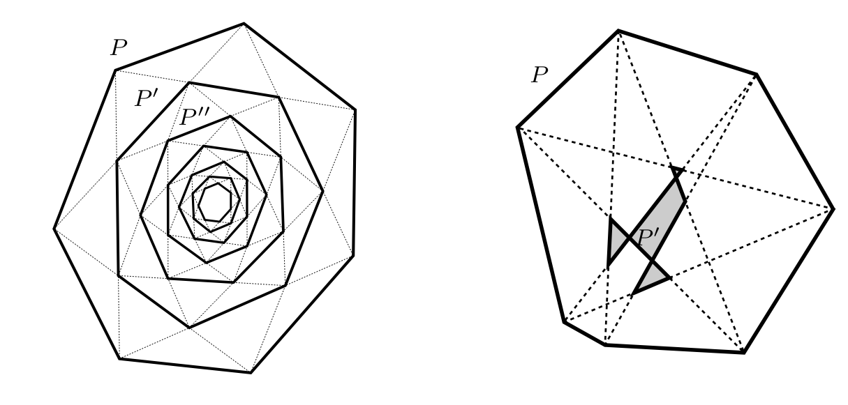
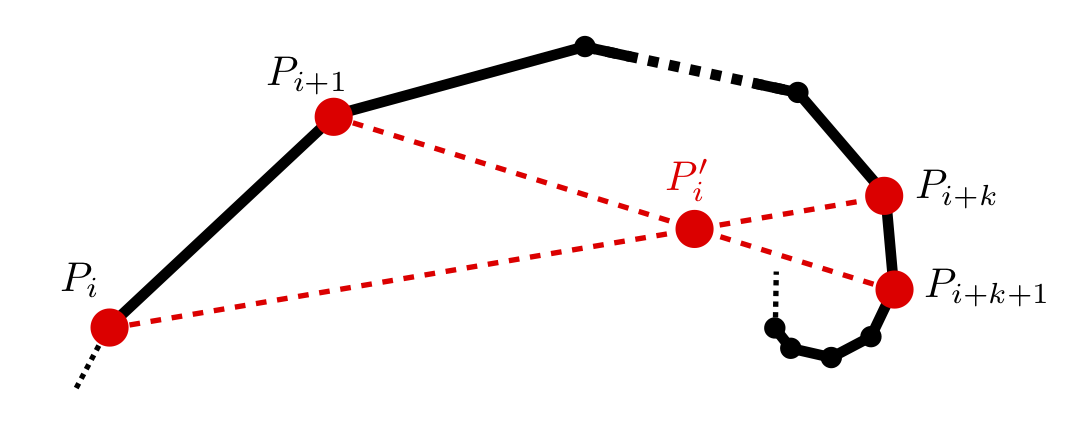
Given a polygon in the real projective plane, let be the map that connects its -th diagonals and intersects them successively to form another polygon whose vertices are given by the following formula:
| (1) |
Figure 1 demonstrates an example of the action of on a convex heptagon. The map is called the pentagram map, a well-studied discrete dynamical system (see [20, 21, 23, 18]). A well-known result is that preserves convexity.111A projective polygon is convex if some projective transformation maps it to a planar convex polygon in the affine patch The -orbit of a convex polygon sits on a flat torus in the moduli space of projective equivalent convex polygons. On the other hand, the geometry of the map is less well-behaved. For , the images of convex polygons may not even be embedded. See Figure 1 for an example of taking a convex heptagon to a polygon that is not even embedded.
Previous results of often had an algebraic and combinatorial flavor, motivated by two branches of studies. The first one was a sequence of works [23, 18, 28, 19] that established that the action on the moduli space of projective convex polygons is a discrete completely integrable system; the second one was M. Glick’s discovery in [5] of the connection between and cluster algebras. In [4], M. Gekhtman, M. Shapiro, S. Tabachnikov, and A. Vainshtein generalized the cluster transformations in [5] to the map acting on so-called “corrugated polygons,” which are polygonal curves in satisfying certain coplanarity conditions. [4] showed that is a discrete integrable system. There are numerous integrability results for these higher-dimensional analogs. See [13, 15, 16, 14, 11]. These led to many applications and connections of to other fields, such as octahedral recurrence [23, 3], the condensation method of computing determinants [23, 6], cluster algebras [5, 4, 7, 3], Poisson Lie groups [2, 10], -systems [12, 3], Grassmannians [1], algebraically closed fields [29], Poncelet polygons [22, 25, 9, 26], and integrable partial differential equations [23, 18, 17].
The geometric aspects of and other deep diagonal maps on planar polygons remain underexplored. There are only a few studies on the geometries of that focused on small or polygons with many symmetries. See [25, 26]. There is no established general framework on the type of geometric properties preserved under for that is analogous to convexity under . Even less is known for geometric objects that have precompact orbits under .
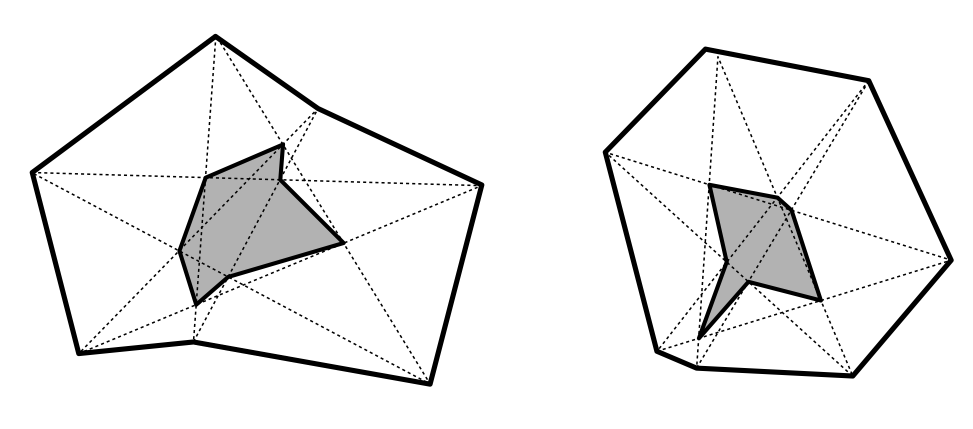
The most relevant result to this endeavor is the discovery of -birds under the map in [27]. A -bird is a planar -gon with , such that there exists a continuous path of polygons connecting to the regular -gon where the four lines
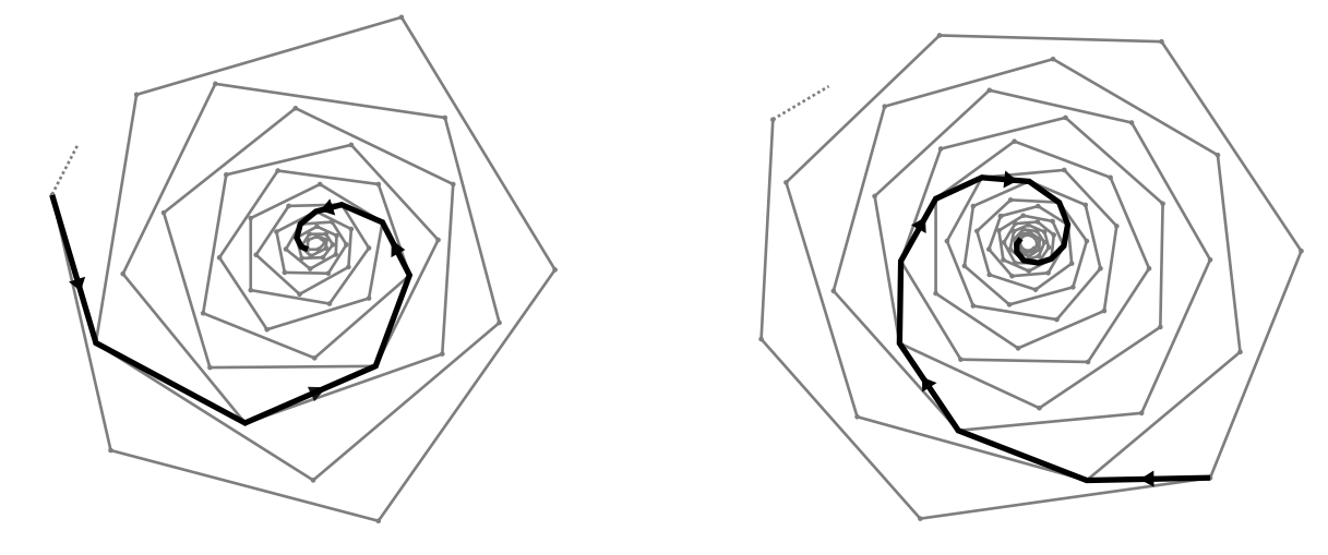
are distinct for all and . The map connects the -th diagonal of a polygon and intersects the diagonals that are clicks apart. See Figure 2 for the action of on 2-birds. In [27], R. Schwartz showed that the -birds are invariant under both and . Experimentally, the -birds seem to have toroidal orbits under , which highly resembles the orbit of convex -gons under . Schwartz also showed that the -birds have precompact forward -orbits modulo affine transformations—a property satisfied by convex -gons under .
This paper has two main results. The first one is the discovery of two classes of geometric objects called type- and type- -spirals that are preserved under for all . These two classes of objects are subsets of twisted polygons: bi-infinite sequences such that no three consecutive points are collinear, and for some fixed projective transformation called the monodromy. The moduli space of projective equivalent twisted -gons is conventionally denoted by . The type- and type- -spirals are the first discovered classes of geometric constructions of that generalize the pentagram map, which provides crucial evidence for a more general understanding of geometrically preserved classes under .
The second result is the precompactness of both forward and backward -orbits of type- and type- -spirals modulo projective transformations for and , a key property satisfied by convex polygons under the pentagram map discovered by Schwartz in [20]. We first examine the action of on type- and type- 3-spirals. We show that one can characterize type- and type- 3-spirals via linear constraints on the corner invariants. We also derive a birational formula of for the corner invariants, which is a generalization of the combinatorial formulas developed by [7]. Then, we present four global invariants under , which we use to prove the precompactness of -orbits modulo projective transformations. For the case , we show that there exists no type- 2-spirals and that the type- 2-spirals are distinct from closed convex polygons. We use the Casimir functions of the -invariant Poisson structure developed in [23] and [18] to show that type- 2-spirals have precompact -orbits modulo projective transformations.
1.2 The -Spirals under the Map
Here we describe the geometric picture of a -spiral. For the formal definition, see 3.1. Geometrically, is a -spiral if for all , we can find a representative such that lies on the affine patch, and the triangles and have positive orientation for all . We call an -representative of .
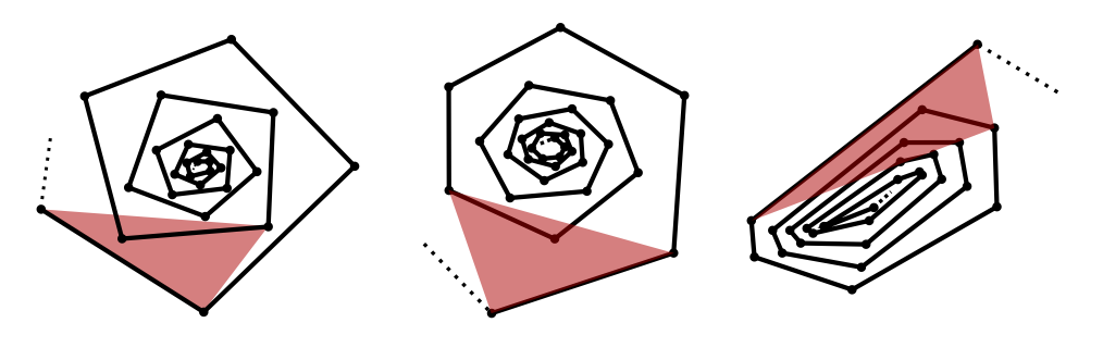
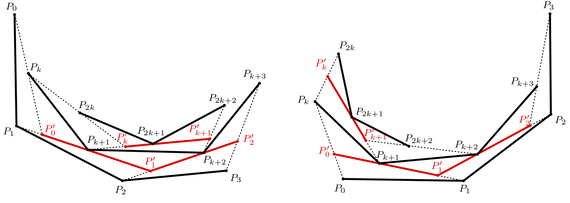
We are mainly interested in two types of -spirals, which we term type- and type- (although there certainly exist many more types of spirals, we only consider these two types here). They are -spirals with additional constraints on the arrangement of the four points , , , . For type- spirals, we require to be contained in the interior of the triangle . For type- spirals, needs to be contained in the interior of . We say is a type- or type- -representative. A class of twisted polygons is a type- -spiral (resp. ) if and only if it admits a type- (resp. ) -representative for all . Let and denote the space of type- and type- -spirals modulo projective equivalence. We will see in 3.1 that they are both open in and hence have dimension . Figure 3 illustrates three examples of representatives of for , and .
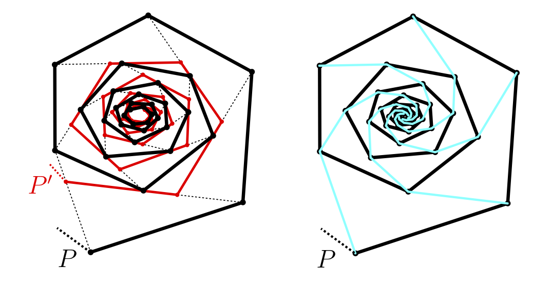
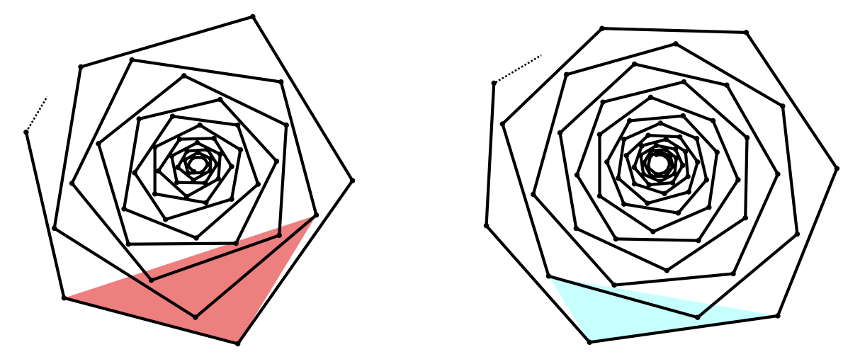
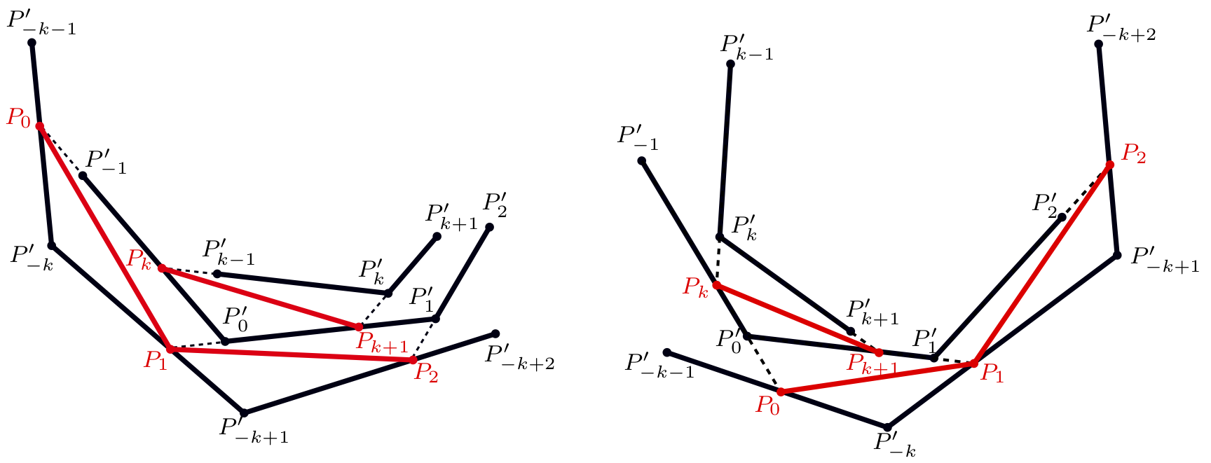
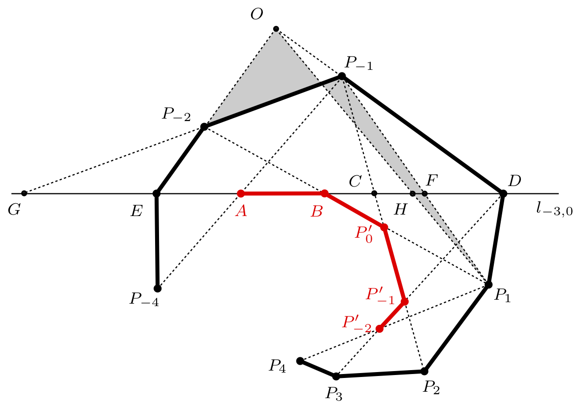
It turns out that and are invariant under both and . Figure 4 shows the inward half of a representative of , with the red arc representing . On the right we have five polygonal arcs by joining vertices of that are 5 clicks apart. We call them the transversals of . One way to distinguish type- and type- spirals is by looking at the orientations of transversals. The transversals of type- spirals are counterclockwise, whereas those of type- are clockwise (See Figure 11). In 3, we use the orientations of these transversals to prove the following main theorem.
Theorem 1.1.
For all and , we have . The same is true for type-.
A key property satisfied by convex polygons under the pentagram map is that the forward and backward orbits of any convex polygon under the pentagram map are precompact modulo projective tranformations. See [20, Lemma 3.2]. Experimental results suggest that the -birds also have precompact -orbits. In [27, Conjecture 8.2] Schwartz conjectured that the -birds have precompact forward -orbits modulo affine transformations. We observed experimentally that and behave analogously under .
Conjecture 1.2.
For and , the forward and backward -orbit of any is precompact in . The same holds for type-.
In 6 and 7, we prove Conjecture 1.2 for and .
1.3 Tic-Tac-Toe Partition and Precompact Orbits
Our main focus will be the case , which we prove in 6.2.
Theorem 1.3.
For , the forward and backward -orbit of any is precompact in . The same holds for type-.
We discovered several interesting properties of the two types of -spirals and the map along our way to prove Theorem 1.3. One major discovery is that the sets and fit well with a local parameterization of introduced by [20] called corner invariants (See 2.4). The invariant sets of under are partitioned by linear boundaries in the parameter space. The boundary lines give a grid pattern that resembles the board of the game “tic-tac-toe.” Each of the four “side-squares” is invariant under .
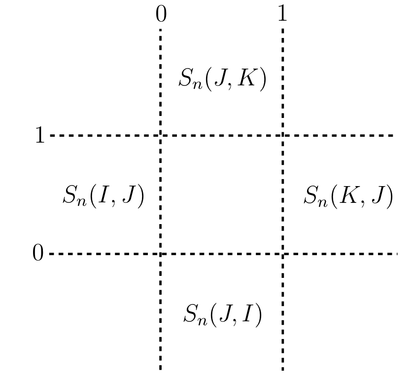
To construct the tic-tac-toe board, consider the three intervals of given by , , . The squares are of the form , , , , etc.. We mark the four side-squares , , , . See Figure 5 for a visualization of the tic-tac-toe grid. Given , we say if all even corner invariants of are in , and all odd ones are in . This means if we plot all pairs of corner invariants onto , we would see points lying in . The other three side squares are defined analogously.
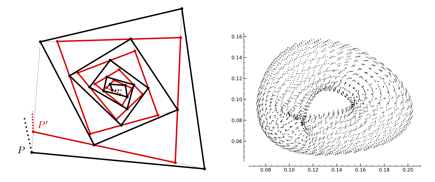
Figure 6 shows vertices of a representative of and the image . On the right, we have the projection of the first iterations of the orbit of under . Each point corresponds to after normalizing to the unit square (here ). We speculate that the orbit lies on a flat torus, where the map acts as a translation on the flat metric.
Twisted polygons that are assigned to these squares have geometric properties. For example, the closed convex polygons always lie in the center square; two of the side-squares are and ; the other two side-squares are obtained by reverting the indexing of vertices of these two types of -spirals. These facts will be proved in 4.
The proof of Theorem 1.3 is algebraic. In 5 I show that is a birational map on the corner invariants, which generalizes a direct application of [7, Theorem 1.6]. For the explicit formulas, see Equation (19). In 6, I derive four algebraic invariants of , which allow me to show boundedness of the corner invariants of the -orbits, thereby proving Theorem 1.3. This approach is reminiscent of Schwartz’s second proof of precompactness of -orbits of convex polygons in [21, Section 3B & 3C].
1.4 The Type- 2-Spirals and Precompact Orbits
We now proceed to the case , where the map is the classical pentagram map. In 3.1 we show that there exist no type- 2-spirals (so Conjecture 1.2 is vacuously true for type- 2-spirals). On the other hand, type- 2-spirals are nontrivial geometric constructions that are distinct from convex polygons. In 7.1, we show that the corner invariants of type- 2-spirals are also partitioned by linear boundaries, and in particular .
We point out that the type- 2-spirals are not related to the pentagram spirals in [24]. The latter requires to be a relabeling of for some positive integer .
In 7.2, we use the Casimir functions of the -invariant Poisson structure on from [23] and [18] to prove Conjecture 1.2 for .
Theorem 1.4.
For , the forward and backward -orbit of any is precompact in .
1.5 Obstacles for and Future Directions
Our algebraic method of proving Theorem 1.3 and 1.4 requires a complete characterization of the corner invariants of and and enough algebraic invariants of that uniformly bound the corner invariants away from the boundaries of and . However, the corner invariants seem to be not partitioned by linear boundaries for , which makes it difficult to analyze the boundaries of the corner invariants of and . Moreover, the map for the corner invariants seems not birational from computer algebra. This makes it difficult to algebraically characterize the corner invariants.
One future direction is to look at the cross-ratio of different combinations of points other than the ones involved in the definition of corner invariants. In 8 we present a conjecture on a potential algebraic invariant of , which can be interpreted as a Casimir function of a Poisson structure over the -parameteris of a quiver . The quiver is associated to a -mesh of type from [7] and is isomorphic to the quiver in [4], which corresponds geometrically to the map .
Another direction is to analyze the two types of -spirals geometrically. There are yet many open problems on the geometry of the two types of -spirals that could hint at the behavior of their -orbits. For open problems, see the end of 3.1. Answering these geometric problems may provide a new approach to tackle Conjecture 1.2.
Finally, for the case , the birational formula for could be applied to other settings such as the action of on Poncelet polygons [26] or discovering -compatible Poisson structures on that generalizes the one in [4] for corrugated polygons.
1.6 Accompanying Program
I wrote a web-based program to visualize the orbits of twisted polygons under . Readers can access it from the following link:
https://zzou9.github.io/pentagram-map/spiral.html
When reaching the website, you will see a representative of a twisted polygon displayed in the middle of the screen. You can click on the user manual button for instructions on how to use the program. I discovered most of the results by computer experiments using this program. The paper contains rigorous proofs of the beautiful pictures I observed from it.
1.7 Acknowledgements
This work was supported by a Brown University SPRINT/UTRA summer research program grant. I would like to thank my advisor, Richard Evan Schwartz, for introducing the concept of deep diagonal maps, providing extensive insights throughout the project, and offering guidance during the writing process. I would like to thank Anton Izosimov and Sergei Tabachnikov for their insightful discussions on the tic-tac-toe partition. Finally, I am grateful to the referees for their helpful comments and for highlighting the connections between the birational formula and the work of Glick and Pylyavskyy.
2 Background
2.1 Projective Geometry
The real projective plane is the space of 1-dimensional subspaces of . Points of are lines in that go through the origin. We say that is a homogeneous coordinate of if the vector is a representative of . Given two distinct points , the line connecting and is the 2-dimensional hyperplane spanned by the two 1-dimensional subspaces. Let be two lines in . The point of intersection is the 1-dimensional line given by the intersection of the two 2-dimensional subspaces. In , there exists a unique line connecting each pair of distinct points and a unique point of intersection given two distinct lines. We call a collection of points in general position if no three of them are collinear.
The affine patch consists of points in with homogeneous coordinate . We call this canonical choice of coordinate the affine coordinate of a point . There is a diffeomorphism given by . We often identify as a copy of in . The line is called the line at infinity.
A map is a projective transformation if it maps points to points and lines to lines and is bijective. Algebraically, the group of projective transformations is , where we are modding by the subgroup and is the identity matrix. We state a classical result regarding projective transformations below with its proof omitted.
Theorem 2.1.
Given two 4-tuples of points and in , both in general position, there exists a unique such that .
The group of affine transformations on is the subgroup of projective transformations that fixes the line at infinity. It is isomorphic to a semidirect product of and . Elements of can be uniquely expressed as a tuple where and . Let denote the subgroup of where iff . These are orientation-preserving affine transformations.
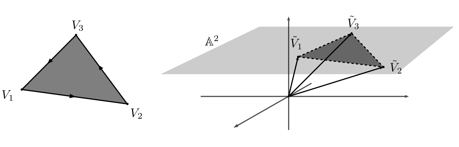
2.2 Orientation of Affine Triangles
Given an ordered 3-tuple of points in or , let denote the interior of the affine triangle with vertices . There is a canonical way to define the orientation of an ordered 3-tuple. Let be the affine coordinate of . We consider the signed area of the oriented triangle, which can be computed as
| (2) |
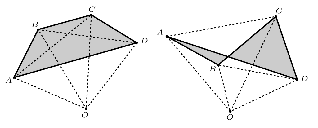
The determinant is evaluated on the matrix with column vectors . We say an ordered 3-tuple is positive if . Figure 7 shows an example of a positive 3-tuple.
Here is another way to compute using the coordinates of :
| (3) | ||||
where the determinant is evaluated on the matrix.
interacts with the action of and the symmetric group on planar/affine triangles in the following way: Given , let . One can show that is positive iff is positive. On the other hand, for all , , so when is a 3-cycle.
Below are useful equivalence conditions for the positivity of . The proof is elementary, so we will omit it.
Proposition 2.2.
Given in general position, and , the following are equivalent:
-
1.
is positive.
-
2.
is positive for some .
-
3.
is positive for all .
-
4.
for some .
-
5.
for all .
2.3 The Cross-Ratio
The cross-ratio is used to construct a projective-invariant parametrization of the -spirals. There are multiple ways to define the cross-ratio of four collinear points on the projective plane, each using its own permutation of the points. We follow the convention used in [20]. Given four collinear points on a line , we choose a projective transformation that maps to the -axis of . Let be the -coordinates of , , , . We define the cross-ratio to be the following quantity:
| (4) |
If lies on the line at infinity, we let . One can check that given any ,
We also define the cross-ratio for four projective lines. Let be four lines intersecting at a common point . Normalize with a projective transformation so that with slopes . We define
| (5) |
with if .
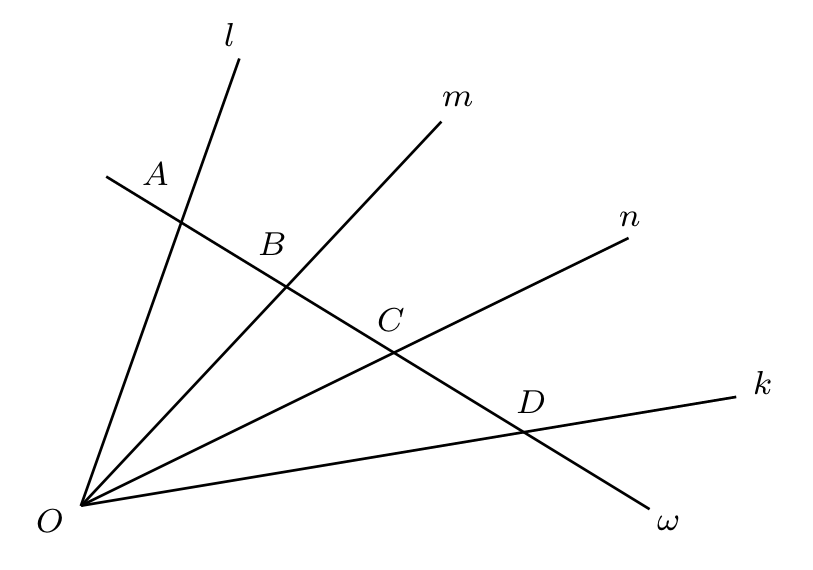
If is a line that does not go through and intersects at respectively, we have
| (6) |
See Figure 8 for the configuration. The proof is elementary, so we will omit it.
2.4 Twisted Polygons, Corner Invariants
Introduced in [23], a twisted -gon is a bi-infinite sequence , along with a projective transformation called the monodromy, such that every three consecutive points of are in general position, and for all . When is the identity, we get an ordinary closed -gon. Two twisted -gons are equivalent if there exists such that for all . The two monodromies and satisfy . Let denote the space of twisted -gons modulo projective equivalence.
The cross-ratio allows us to parameterize with coordinates in . Given a twisted -gon , the corner invariants of is a coordinate system given by
| (7) |

See the left side of Figure 9 for a geometric interpretation of the corner invariants. Let . By Equation (5), the corner invariants can be computed by
| (8) |
See the right side of Figure 9 for the line configurations.
Since is invariant under projective transformations, for all we have , so a -tuple of corner invariants is enough to fully determine the projective equivalence class of a twisted -gon. We use to denote the corner invariants of without adding square brackets around . To obtain the corner invariants of , one can simply choose an arbitrary representative and compute its corner invariants. [23, Equation (19) & (20)] showed that one can also revert the process and obtain a representative twisted polygon of the equivalence class given its corner invariants.
3 The Spirals and -Orbit Invariance
In this section, we explore the geometric properties of type- and type- -spirals and prove Theorem 1.1. In 3.1, we give rigorous definitions of the two types of -spirals and discuss their geometric properties. In 3.2, we introduce a construct associated to the two types of -spirals called the transversals. In 3.3 and 3.4, we prove Theorem 1.1 using geometric properties of the transversals.
3.1 The Geometry of -Spirals
Here we give the formal definition of a -spiral and its two subsets called type- and type-. We then explore their geometric properties and present some open problems.
Definition 3.1.
Given integers , , we say that is a -spiral if for all , there exists a representative that satisfies the following: For all , lies in , is positive, and is positive. Such a representative is called an -representative. Saying that is a -spiral means that admits an -representative for all .
Remark 3.2.
The idea of considering an -representative for each is new to the literature and may at first seem superfluous. Readers will see in 4 that this condition is natural when we examine the corner invariants of the two types of -spirals. See the end of this section for open problems related to the geometry of -representatives.
In practice, since is a twisted -gon, it suffices to find a single -representative for some . One can then obtain other -representatives for by applying the -th power of the monodromy of to , where .
Definition 3.3.
A -spiral is of type- or type- if for all , it has an -representative that satisfies the following conditions:
-
•
is of type- if for all ;
-
•
is of type- if for all .
See Figure 10 for 0-representatives of type- and type- 6-spirals. For the type- -spirals, we show that positivity of is equivalent to positivity of . The latter condition turns out to be more convenient for showing invariance.
Proposition 3.4.
is a type- -spiral if and only if for all , there exists a representative that satisfies the following: for all , lies in , is positive, is positive, and .
Proof.
Since , we see that is nonempty, so the three points , , are in general position. It then follows from Proposition 2.2 that is positive iff is positive. ∎
Corollary 3.5.
There exists no type- 2-spirals.
Proof.
It suffices to show that there exists no configuration of four points such that , are both positive and . If is positive and , then Proposition 2.2 implies is positive, but that contradicts positive because . ∎
On the other hand, type- 2-spirals do exist. Geometrically, their -representatives look like triangular spirals. See 7 for a more thorough discussion on type- 2-spirals.
Remark 3.6.
One may attempt to define the two types of -spirals on bi-infinite sequences of points in with no periodicity constraints. The results in this section hold true for this more general definition. We restrict our attention to twisted polygons because it’s a finite-dimensional space, which allows us to more easily keep track of the -orbits.
We now proceed to discuss some geometric properties of type- and type- -spirals. A twisted polygon is called -nice if the four points are in general position for all . The -nice condition is projective invariant. Let denote the space of -nice twisted -gons modulo projective equivalence.
Proposition 3.7.
For all , is open in , so it has dimension .
Proof.
The condition that four points are in general position remains true if we perturb one of the points in a small enough neighborhood of . The dimension of comes from the fact that has dimension , which is shown in [18, Lemma 2.2]. ∎
Proposition 3.8.
Both type- and type- -spirals are -nice.
Proof.
We give a proof to the type- case. The type- case is analogous, so we will omit it. Given a type- -spiral and an integer , let be an -representative of . Since is positive, these three points cannot be collinear. Also, since , does not lie in any of the lines joined by two of the three vertices . This shows that are in general position. ∎
As stated in 1.2, we let and denote the space of type- and type- -spirals (By Corollary 3.5, for all ).
Proposition 3.9.
Both and are open in , so they both have dimension .
Proof.
The positivity conditions of and are open conditions from continuity of the determinant function. The condition for type- (or for type-) is equivalent to the positivity of certain determinants by Proposition 2.2, so this is also an open condition. Finally, and follows from Proposition 3.8. ∎
A twisted polygon is closed if there exists some positive integer such that , or with identity monodromy. We show that neither type- nor type- -spirals are closed.
Proposition 3.10.
For all and , if , then is not closed. The same holds for .
Proof.
Given any closed -gon on , let be the convex hull of the vertices of . Since has finitely many vertices, there exists a vertex such that . Then, since , we must have . It follows that is not an -representative of type- -spiral for any or . The proof for type- is similar, so we omit it. ∎
The two types of -spirals seem to possess rich geometric properties. We will present some open problems. In the discussion below, denotes a type- or type- -spiral.
Problem 3.11.
For all , is it always possible to find -representatives such that for all , is positive (in other words, always lies on the same side of the line )?
Problem 3.12.
Let be an arbitrary representative of . Is there a minimal such that is an -representative on some affine patch of ? Does there exist that is an -representative for all ?
Problem 3.13.
Given an -representative , does converge to a point in as ?
3.2 Transversals of the Spirals
In this section, we prove our remark in 1.2 that transversals for type- spirals are oriented counterclockwise, whereas transversals for type- are oriented clockwise. Recall that the transversals of an -representative of a -spiral are polygonal arcs joined by vertices for . See Figure 11 for one of the transversals of the two representatives from Figure 10.
Lemma 3.14.
Given (See Figure 12) such that , , , are all positive. Then, is positive iff is positive.
Proof.
For the forward direction, normalize with so that and . Let , , and . Since is positive, Equation (3) gives us
Similarly, positivity of and give us . Next, observe that
Since , we have , which implies
This shows positivity of .
The proof for the backward direction is analogous. Normalize so that and . Let , , . Positivity of , , and implies . One can then check that
This shows positivity of . ∎
The next proposition formalizes our claim on the orientation of transversals.
Proposition 3.15.
Let be an -representative of a -spiral . For all , if is type-, then is positive; if is type-, then is positive.
Proof.
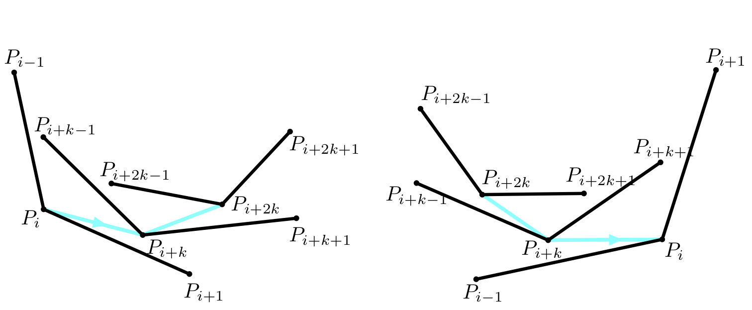
The proof applies Lemma 3.14 with suitable choices of . See Figure 13 for the configuration of points involved.
We start with of type-. Consider the following choices of vertices:
It follows immediately from the definition of a type- -representative that and are positive. The other conditions follow from applications of Proposition 2.2. Apply Proposition 2.2 with positive and to get positivity of . Apply Proposition 2.2 with positive and to get positivity of . Apply Proposition 2.2 with positive and to get positivity of . Then, the backward direction of Lemma 3.14 implies is positive.
The proof for type- is analogous. Consider the following choices of vertices:
Positivity of and follows from the definition of a type- -representative. A similar application of Proposition 2.2 as in the case of type- gives positivity of , , and , which we will omit. Finally, the forward direction of Lemma 3.14 implies is positive. ∎
3.3 Invariance of Forward Orbit
In this section, we prove that and are -invariant. We will use Equation (1) for our labeling convention. See Figure 14.
If is -nice, then is always well-defined. In particular, Proposition 3.8 implies is well-defined on and .
Remark 3.16.
doesn’t necessarily send -nice twisted polygons to -nice twisted polygons. Here is an example provided by the anonymous referee: Fix . Consider the function mapping . One can check that is a -nice twisted -gon for any with monodromy that is a scale-rotation, but is the zero function and hence not -nice. What we will show is that in the case of type- and type- -spirals, does preserve -niceness. This is a direct consequence of Theorem 1.1 and Proposition 3.8.
We proceed to prove the -invariance of and separately. We start with the following lemma.
Lemma 3.17.
Given four points in in general position with . Let . There exist and such that
Proof.
Since , there exists such that
Taking and gives us the desired result. ∎
Proposition 3.18.
For all and , .
Proof.
Given an -representative of some , we will show that is a type- -representative of by proving that for all , is positive, is positive, and . See the left side of Figure 15 for configurations of relevant vertices of and .
Let be fixed. Since is a type- -representative, for all . Applying Lemma 3.17 with Equation (1) on for gives us
| (9) | ||||||
where and . In particular, this shows , so the three points are in general position.
To see that is positive, Equation (3) and (9) give us
| (10) | ||||
Then, since and , Proposition 2.2 implies , so .
Next, we show that . Let and . (9) implies and
It follows that
Observe that the coefficients , , are all in and sum up to , so .
Finally, using Equation (3) and (9), we have
| (11) | ||||
Proposition 3.15 implies , so Since are in general position and , Proposition 2.2 and Equation (11) imply . We conclude that is a type- -representative. ∎
Proposition 3.19.
For all and , .
Proof.
The proof is analogous to the one for Proposition 3.18. Replacing with , we may work with the setup in the proof of Proposition 3.18. See the right side of Figure 15.
The key difference between type- and type- is that conditions for type- -spirals give us the following linear relations when we apply Lemma 3.17 with (1) on for :
| (12) | ||||||
where and . We can see that , so the three points are in general position.
A very similar computation as Equation (10) shows positivity of , so we will omit it. Next, let and . Notice that , , and are all in and sum up to . Also, Equation (12) implies
This shows . Finally, positivity of follows from a similar computation as Equation (11), , the points are in general position, and Proposition 2.2. ∎
3.4 Invariance of Backward Orbit
In this section, we complete the proof of Theorem 1.1 by showing that and are -invariant. One can derive a formula for from Equation (1). Given any -nice twisted -gon , is given by
| (13) |
Proposition 3.8 implies is well-defined on and . In general, needs not preserve -niceness of twisted polygons.
Proposition 3.20.
For all and , .
Proof.
Given a type- -representative, we will show that is a type- -representative by proving that for all , is positive, is positive, the four points are in general position, and . See the left side of Figure 16 for configurations of relevant vertices of and .
Let be fixed. Since is a type- -representative, we must have for all . Applying Lemma 3.17 with Equation (13) on for gives us
| (14) | ||||||
where and .
We first show that is positive. From Equation (14) we have
It follows that , so is positive.
Next, we show that . Let and . Equation (14) implies and
Observe that the coefficients , , and are all in and sum up to 1, so .
Finally, we check is positive. We aim to invoke Lemma 3.14 with the following choices of vertices:
| (15) |
Positivity of is a direct consequence of the above argument. Positivity of follows from positivity of , , and Proposition 2.2. Next, observe that
| (16) | ||||
Then, positivity of and follows from positivity of and . To see that is positive, apply Proposition 2.2 on positive and to get positive. The backward direction of Lemma 3.14 then implies is positive. We conclude that is a type- -representative. ∎
Proposition 3.21.
For all and , .
Proof.
The proof is similar to that of Lemma 3.20 (See right side of Figure 16). We will point out some key differences. Replacing with , we may work with the setup in the proof of Proposition 3.20. Applying Lemma 3.17 with (13) on for gives us
| (17) | ||||||
where and . Positivity of follows from a similar computation as in (3.4). Next, let and . Equation (17) implies
Observe that the coefficients , , and are all in and sum up to 1, so .
Finally, assign to be the same vertices as in (15). Positivity of , , , , and follows from a very similar proof as that of Proposition 3.20, with (16) replaced by
The backward direction of Proposition 3.14 then implies is positive. ∎
We conclude this section by stating that Proposition 3.18, 3.19, 3.20, 3.21 together prove Theorem 1.1.
4 Coordinate Representation of 3-Spirals
4.1 The Tic-Tac-Toe Grids
Recall the intervals , , from 1.3. One can partition into a grid. See Figure 5. We make the following definition:
Definition 4.1.
For , let be the subset of that satisfies the following: given , for all , . We similarly define , , and .
The following symmetries of the four grids follow directly from Definition 4.1.
Proposition 4.2.
For , define the map by . Define the map by . Given , the following are true:
-
•
If , then for all . This also holds for , , and .
-
•
if and only if .
-
•
if and only if .
To understand the geometry implied by the corner invariants, we need to examine what happens when the corner invariants take value from .
Proposition 4.3.
For all with corner invariants and , we have the following correspondence between the position of and the values of and :
| Configuration | Coordinates | Configuration | Coordinates |
|---|---|---|---|
Proof.
Consider the following lines:
See Figure 17 for a visualization of the configurations of points and lines. Equation (8) implies and . This yields
| Configuration | Lines | Coordinates | Configuration | Lines | Coordinates |
|---|---|---|---|---|---|
which is precisely the relationship described in the proposition. ∎
Remark 4.4.
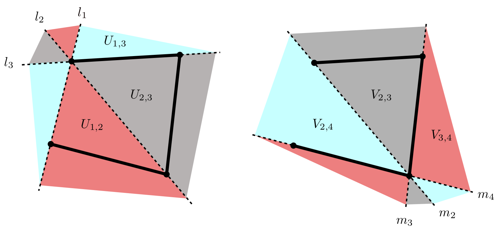
Proposition 4.3 also gives us a way to determine the position of when neither nor takes value in . Suppose the four points are in general position. For distinct, we define to be the connected component of that does not intersect . For distinct, we define to be the connected component of that does not intersect . See Figure 18 for a visualization of the ’s and ’s using the point configurations given in Figure 17. By Proposition 4.3 and continuity of , we have the following:
| Configuration | Coordinates | Configuration | Coordinates |
|---|---|---|---|
Corollary 4.5.
Given with corner invariants , if for all , then is -nice. Moreover, every four consecutive points of are in general position.
Proof.
Using Proposition 4.3 we may check that
| Collinearity | Coordinates | Collinearity | Coordinates |
|---|---|---|---|
| , , | , , | ||
| , , | , , | ||
| , , | , , | ||
| , , |
All seven cases contradict the assumption in the corollary. Therefore, the four points , , , are in general position, and the four consecutive points , , , are in general position for all . This shows is 3-nice, and every four consecutive points of are in general position. ∎
Our goal of this section is to prove the following correspondence theorem:
Theorem 4.6.
For all , , .
This theorem immediately produces the following important corollary.
Corollary 4.7.
For all , the four cells , , , are both forward and backward invariant under .
Proof.
The case and follows immediately from Theorem 1.1 and 4.6. We will prove the case . The case is completely analogous, so we will omit.
Fix . Recall the maps and from Proposition 4.2. Equation (1) implies . Then, Proposition 4.2 implies , so . Finally, observe that
It follows that . We omit the proof of . ∎
4.2 The Correspondence of and
Here we show that is equivalent to . We will first show that the corner invariants of a -representative of some satisfies . Then, we will show that we can find type- -representatives for all given any .
Lemma 4.8.
If is an -representative of , then for all .
Proof.
Since is positive, we may normalize with so that , , and . Let . It suffices to show that , , and . We get from positivity of , and we get from positivity of . Finally, since is positive and , Proposition 2.2 implies is positive, which gives us as desired. ∎
Proposition 4.9.
For all , .
Proof.
Fix . Let be an -representative of with corner invariants . Normalize with so that , , and . Let denote the slope of the line . See Figure 19 for the configuration of points.
We want to show that . By Lemma 4.8, . This implies . On the other hand, since , we have , and . This gives us
This concludes the proof. ∎
Proposition 4.10.
For all , .
Proof.
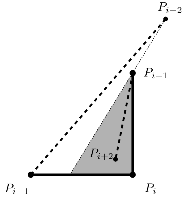
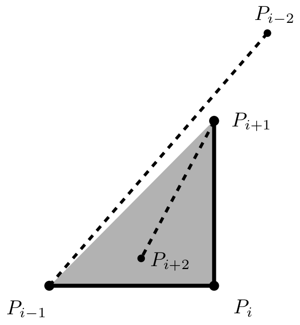
Proposition 4.9 implies we only need to show . Given , let be a representative that satisfies , , , . Say that satisfies condition if the three triangles , , are all positive, , and .
We show that for all , if satisfies , then satisfies . Since is positive, we can normalize with so that , , and . Let denote the slope of . Since , we know that . Then, implies . This gives us . On the other hand, implies . Since , this is equivalent to , which implies . Thus, the two lines and must meet in the shaded triangle in Figure 19, which implies , are positive, , and , so satisfies . Finally, since clearly satisfies , by induction satisfies for all , so is a type- -representative of a 3-spiral. We conclude that . ∎
4.3 The Correspondence of and
Here we show that is equivalent to . The ideas behind the proofs are essentially the same as the ones in 4.2. We will focus on explaining how to modify the details of the proofs in 4.2 for type- 3-spirals and .
Lemma 4.11.
If is an -representative of , then the quadrilateral joined by vertices is convex for all .
Proof.
Normalize with so that , , , and . Positivity of and implies and . Positivity of , , and Proposition 2.2 shows . ∎
Proposition 4.12.
For all , .
Proof.
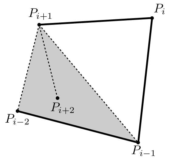
Let be a -representative of with corner invariants . Lemma 4.11 implies the quadrilateral is convex. Next, since is a type- -representative, for all (See Figure 20). Referring back to Remark 4.4, convexity of implies doesn’t go through , so whenever . ∎
Lemma 4.13.
Given a -nice sequence and an integer , let and be the corner invariants of . If the following conditions are true:
-
•
and are both positive;
-
•
The quadrilateral is convex;
-
•
.
Then, the following hold:
-
•
;
-
•
The quadrilateral is convex;
-
•
and are both positive.
Proof.
Recall that from the proof of Proposition 4.12, we claimed that if the quadrilateral is convex, then the line doesn’t go through . Since , Remark 4.4 implies , in which case all conclusions of this lemma will hold. See Figure 20 for a visualization of the five points. ∎
Proposition 4.14.
.
Proof.
Proposition 4.12 gives us , so we show the other containment. Given , we can find a representative that satisfies , , , . Corollary 4.5 shows that is 3-nice. To see that , are positive, and , we may inductively apply Lemma 4.13. This implies . ∎
5 A Birational Formula for
Given two spaces and , a rational map is an equivalence class of maps where is a dense open in , and the equivalence relation is given by if they restrict to the same map on . A map is birational if there exists a rational map such that restricts to the identity on a dense open of and restricts to an identity on a dense open of .
In this section, we show that is a birational map by finding an explicit formula using the corner invariants.
5.1 The Formula
Let be a twisted -gon, and . In this section, we use a different labeling convention:
| (18) |
We let and denote the corner invariants of and respectively. Our goal is to show that is a birational map over the corner invariants. I discovered it using computer algebra and the reconstruction formula in [23, Equation (19)].
Proposition 5.1.
Given , the following formula holds (indices taken modulo ):
| (19) |
One can verify Equation (19) with the following procedure: Given the corner invariants of , use the reconstruction formula from [23, Equation (19)] to obtain a representative . Apply on as in Equation (18) to get . Then, compute the corner invariants of . We present a geometric proof of Equation (19) using cross-ratio identities. We start with the following lemma, which is a classical observation in projective geometry called “quadrangular sets.”
Lemma 5.2.
Let be four points in general position, and let be a line that contains none of the four points. For all , let and Then,
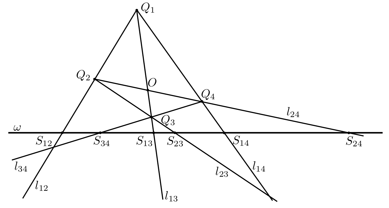
Proof.
Let . See Figure 21 for an example of the point configurations. Applying Equation (6) on with respect to and gives us
Next, applying Equation (6) twice on with respect to and gives us
Combining the above two equations completes the proof. ∎
Proof of Proposition 5.1.
From the symmetry of Equation (19), it suffices to prove the formula for . That is,
| (20) |
Let and . We label points as follows:
| (21) |
Since , every five consecutive points of are in general position. This ensures that point and the points in Equation (21) are all distinct. See Figure 22 for a visualization of the assignment of labels to these points.
It follows from Equation (7) that . Using Equation (8), we have
| (22) | ||||
We may further invoke Lemma 5.2 with , , , , and . This gives us
| (23) |
The rest of the proof is just algebraic verification. Normalize with a projective transformation so that is the -axis of . Let , , , , , , , be coordinates of , , , , , , , respectively. Plugging (22) and (23) into the numerator of (20) gives us
The denominator can be computed similarly. We skip the computation and list the results:
Combining the above two equations gives us
which is precisely Equation (20). ∎
Next, we provide a formula for the inverse of .
Proposition 5.3.
The map is birational. Its inverse is given by
| (24) |
We will give an algebraic proof. Consider two families of rational maps and . Write and . Then, we set
| (25) |
Lemma 5.4.
Let be the map given by
| (26) |
Then, is an involution. Moreover, when is odd, and .
Proof.
To see is an involution, a direct computation shows that
Next, we show that when is odd, . We will show by direct computation that is the identity on the -th coordinate when is even. First, when is even, . The -th coordinate of is given by
This is precisely what we want. One can similarly carry out the computation of for the -th coordinate, and odd. We will omit these heavy computations and conclude that . Finally, to see , observe that is odd iff is odd. Therefore, is the identity map by the previous argument. The same argument shows that is the identity. ∎
The following corollary is immediate. We omit the proof.
Corollary 5.5.
For all such that is odd, and are birational maps.
Proof of Proposition 5.3.
We first claim that . We will provide the computation for even coordinates. Let denote the image of under , and let denote the image of under . Then, we have
Observe that this is precisely the first line of (19). The computation for is analogous, thus omitted. Then, by Corollary 5.5, . Finally, Equation (24) follows from a direct computation of using Equation (25), which we will omit. ∎
5.2 Conjugated Corner Invariants and Its Formula
To relate Equation (19) to parameters in [7], it is convenient to consider another coordinate system of , which we define below.
Definition 5.6.
Given , define the conjugated corner invariants to be coordinate functions given by .
The conjugated corner invariants can be viewed as the image of the corner invariants under a birational map sending each coordinate . Observe that restricted to the dense open set is the identity map, so is also a coordinate system for . Geometrically, the map corresponds to a different choice of permutation in the cross-ratio.
Throughout this section, we will use and to denote the conjugate corner invariants of and . We start by observing some symmetries of conjugating our factorization maps and from Equation (25).
Lemma 5.7.
For all , we have .
Proof.
We can check this by direct computation. We show that the equation holds on even coordinates. The -th coordinate of is given by
The -th coordinate of is given by
which is precisely the -th coordinate of . The computation for the odd coordinates is similar. ∎
Since is an involution, it immediately follows that . This allows us to obtain a formula for with respect to the conjugated corner invariants.
Proposition 5.8.
Given any 3-nice twisted -gon , the following formula holds (indices taken modulo ):
| (27) |
Proof.
From the proof of Proposition 5.3, we saw that the formula for on the corner invariants is given by . It follows that the formula for conjugated corner invariants is . By Lemma 5.7,
It remains to check that agrees with Equation (27). The -th coordinate of is given by
This is precisely from Equation (27). The computation for odd coordinates is omitted. ∎
Using Lemma 5.4, we can easily compute the formula of with respect to the conjugated corner invariants. The proof is again a direct computation, so we omit it.
Corollary 5.9.
The formula for with conjugated corner invariants is given by . More specifically,
| (28) |
5.3 Relation to -Variables
In this section, we discuss how Equation (18) generalizes the results from [7]. The propositions in this section hold for all four cells , , , . For notational convenience, our statements will only mention . The readers may assume that the propositions hold for the other three cells with the same proof.
The map along with the labeling convention of Equation (18) corresponds to the following construction in [7]. Let be distinct and assume . Say that is a -pin if and the vectors , , generate all of .
Definition 5.10 ([7, Definition 1.4]).
Let be a -pin and suppose . A -mesh of type and dimension is a grid of points in with which together span all of and such that
-
•
, , , are distinct for all .
-
•
Let . Then, , , , all lie on for all .
-
•
The four lines , , , (all of which contain ) are distinct for all .
Let , which is a -pin. Given a representative of some , we can consider a grid where is the -th vertex of .
Proposition 5.11.
is a -mesh of type and dimension 2.
Proof.
The first two conditions of Definition 5.10 are straightforward to verify using the identification from Proposition 4.10. For the third condition, let . Then, we have
Notice also that and , so 3-niceness of implies they are distinct. The other pairings are distinct because of 3-niceness of . ∎
[7] then introduces the parameters associated to a -mesh. Fix a -pin and a -mesh of type and dimension . For all , consider
| (29) |
See the left side of Figure 23 for the setup using the -mesh from Proposition 5.11. [7, Theorem 1.6] give us the following relation on :
| (30) |
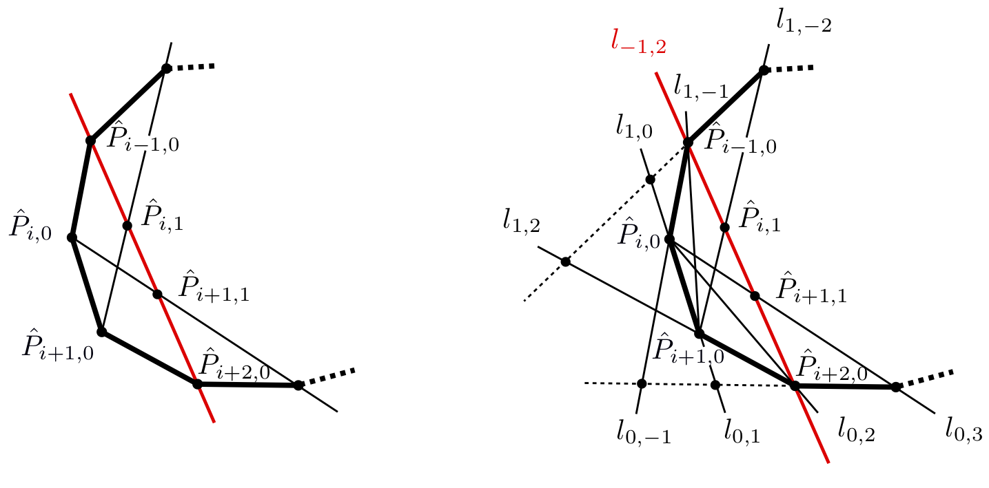
Lemma 5.12.
Given a representative of with conjugated corner invariants . Let be its corresponding -mesh with for all . Then, for all ,
| (31) |
Proof.
Let . See right side of Figure 23 for the setup. Equation (8) gives us
Notice that . Then, from elementary cross ratio identities we have
which is precisely Equation (31). ∎
Remark 5.13.
Equation (31) is very similar to the correspondence of and corner invariants in the case. Let be an arbitrary twisted -gon with . If we use the labeling convention , then the -orbit , where is the -th vertex of , is a -mesh of type . Denote by the corner invariants of . Then, for all ,
| (32) |
For the proof of Equation (32), see [5, Equation (2.2)].
Theorem 5.14.
For the -pin , the transformation formula of from [7, Theorem 1.6] is a direct consequence of the birational formula for the conjugated corner invariants under .
Proof.
It suffices to show that we can use Equation (31) to derive (30) for . We first compute and using Equation (27) and (28):
| (33) | ||||
It follows that
This concludes the proof. ∎
6 The Precompactness of Orbits
In this section, we establish four algebraic invariants of . We then use them to prove Theorem 1.3. Having Theorem 4.6 in hand, we may fully work with and . Our strategy is to use the algebraic invariants to show that the corner invariants are uniformly bounded.
6.1 The Four Invariants
Proposition 6.1.
Given with corner invariants , consider the following four quantities :
| (34) |
Then, is invariant under for .
Proof.
We first show that is invariant under . Let denote the invariants obtained by plugging in from Equation (24). Observe that
This shows . Next, we show that and are invariant. Using conjugated corner invariants, we see that and . We let be the first invariant of . Equation (27) gives us
where the last equality follows from cyclically permuting the numerator. This shows . The proof for goes through the same computation, so we omit it.
Finally, observe that , so by invariance of , we know that must also be invariant. This concludes the proof. ∎
Remark 6.2.
As shown in the proof of Proposition 6.1, and correspond to the product of conjugated corner invariants. is the ratio of the two Casimirs of the invariant Poisson structure on . For discussions on and the Casimirs, see [26, 2.3]. Also, since , the four invariants are not algebraically independent.
Below is a direct consequence of the invariance of the ’s. Since the ’s are preserved by the forward action, it must also be preserved by the backward action.
Corollary 6.3.
The four invariants are also invariant under .
6.2 Proof of Theorem 1.3
Recall that a subset of a topological space is precompact if the closure of is compact. To show that the -orbit is precompact, it suffices to show that the corner invariants of the orbit are uniformly bounded away from the singularities .
In this section, we let . Given , for all , let whenever exists. Let for . By Proposition 6.1, is independent of . All sequences are indexed by unless specified otherwise. Finally, when we say “ converges/diverges on a subsequence, and converges/diverges on the same subsequence,” we mean that a subsequence of with the same choice of indices as the subsequence of converges/diverges.
Lemma 6.4.
Given , there exist such that for all and .
Proof.
We first claim that for each , the sequence is bounded above uniformly by some . If not, then on a subsequence, which implies on the same subsequence. Since for all , we must have and for all . This implies on the same subsequence, but that contradicts invariance of . Therefore, is bounded above by . Taking satisfies the condition in the lemma.
Next, we show is bounded below uniformly by some . If not, then on a subsequence, so on the same subsequence. From the argument above, for all and , which gives us , so the sequences are uniformly bounded for all . This together with on a subsequence implies on the same subsequence, but that contradicts invariance of . Therefore, is bounded below by . Taking completes the proof. ∎
Lemma 6.5.
With the same notation as in Lemma 6.6, there exist such that for all and .
Proof.
We first claim that for each ,the sequence is bounded above uniformly by some . If not, then, on a subsequence. Since for all , we must have on the same subsequence, but that contradicts invariance of .
Next, we show that is bounded below uniformly by some . If not, then a subsequence of must diverge, so the same subsequence of also diverges. Lemma 6.4 and together implies diverges on the same subsequence, but that contradicts invariance of . Finally, taking and completes the proof. ∎
The proofs of the following two lemmas are analogous to Lemma 6.4 and 6.5. We will omit the details and point out which invariants to use in each step.
Lemma 6.6.
Given , there exist such that for all and .
Proof.
For each , the sequence is bounded below by some , for otherwise diverges on a subsequence. Next, since is bounded below by , is bounded above by some . Taking and completes the proof. ∎
Lemma 6.7.
With the same notation as in Lemma 6.6, there exist such that for all and .
Proof.
For each , the sequence must be bounded below by some , for otherwise on a subsequence. It’s also bounded above by some . To see this, Lemma 6.6 implies all corner invariants are bounded away from 0, so if is not bounded above, then diverges on a subsequence. Taking and completes the proof. ∎
Proof of Theorem 1.3.
We will show that the forward orbit of has uniformly bounded corner invariants. By Proposition 4.10, . Let , be compact intervals derived from Lemma 6.4 and 6.5. Then, the sequence is contained in , so it is uniformly bounded. To show precompactness of the backward orbit of , one can adapt the proofs of Lemma 6.4 and 6.5 with very few changes. We omit the details. The case follows from Lemma 6.6 and 6.7 by essentially the same argument, which we again omit. ∎
7 Type- 2-Spirals and Precompact Orbits
7.1 The Corner Invariants of Type- 2-Spirals
We finish this paper by discussing the type- 2-spirals. Proposition 3.10 implies is disjoint from the moduli space of closed convex polygons, so is a new invariant geometric construction under the pentagram map by Theorem 1.1. In this section, we analyze the corner invariants of and show that just like the type- and type- 3-spirals, it is cut out by linear boundaries.
Proposition 7.1.
For all , given any with corner invariants , we have and for all .
Proof.
Let be an -representative of . Normalize by so that , , on the affine patch, which is possible because is positive. Let denote the slope of . Positivity of and implies and . Similarly, since , we have and . It follows that
| (35) | ||||
This concludes the proof. ∎
Proposition 7.2.
For all , if has corner invariants such that and for all , then .
Proof.
Fix . Let be a representative of such that , , , and . We say satisfies condition if is positive and . Then, is a type- -representative of 2-spirals iff satisfies for all . Notice that satisfies , so by an induction argument, it suffices to show that for , if satisfies , then satisfies .
If satisfies , then is positive. Normalize by so that , , and . We will use the same notation and as Proposition 7.1. Since , we have and . Then, since and , Equation (35) gives us
It follows that and . The latter inequality implies , so in particular and hence . The two conditions and implies and positive, so satisfies as desired. We conclude that . ∎
7.2 The Precompactness of Orbits
We adapt the argument for Theorem 1.3 to give a quick proof of Theorem 1.4 using the Casimir functions of the -invariant Poisson structure on that were developed in [23, Theorem 1.2]. One can find the proof of the following lemma in [23, 2.2].
Lemma 7.3.
For the map acting on a twisted -gon with corner invariants , one has the following four invariant quantities.
We continue to use the notation from 6.2. In addition, we write . We define , , and analogously. By Lemma 7.3, the values of these four quantities are independent of the choice of .
Lemma 7.4.
For all , given , there exists such that for all and .
Proof.
Fix . We first show that is uniformly bounded above by some . Since for all , we must have . Then, if on a subsequence, also diverges on the same subsequence, but that contradicts invariance of . This implies for some . Taking satisfies the condition in the lemma.
Next, we show that is uniformly bounded below by some . We first notice that . This implies if on a subsequence, then on the same subsequence, but that contradicts invariance of . Therefore, for some . Taking completes the proof. ∎
Lemma 7.5.
For all , given , there exists such that for all and .
Proof.
The argument is analogous to the proof of Lemma 7.4. Fix . To find that bounds uniformly from below, we use the fact that . We then set . To find that bounds uniformly from above, we use the fact that . We then set to complete the proof. ∎
Lemma 7.4 and 7.5 together implies that the forward -orbit of any is precompact in . One can use the same argument to show that the backward -orbit is also precompact. We have thus completed the proof of Theorem 1.4.
8 Appendix
8.1 Conjectures for Invariants
Given , we may consider the following quantity:
| (36) |
When is well-defined, we write , or simply if the value of is clear from the context. Let (or simply ) denote the product .
Proposition 8.1.
For all , given , there exists , , such that
| (37) |
for all . The same holds for .
Proof.
The grid where is the -th vertex of is a -mesh of type with for . The proof is essentially the same as the one for Proposition 5.11, so we will omit it. Then, from [7, Theorem 1.6], we have
| (38) |
It follows that
| (39) | ||||
This implies for all . Taking completes the proof. ∎
Remark 8.2.
Combining the results of [7] and [4], we see that Proposition 8.1 is equivalent to [4, Theorem 2.1]. Specifically, the quantity in Equation (37) is shown to be a Casimir function with respect to a Poisson structure that is invariant under the -variable transformation of a quiver , which we will define below.
Consider the infinite directed graph whose vertices are indexed by , with directed edges , , , and for all . See Figure 25 for a visual representation of this quiver. We refer the readers to [7, 9] for the construction of this quiver and the proof that the -variable transformations satisfy (38).
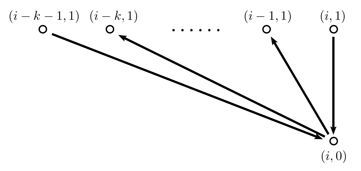
For all , the -variables corresponding to are periodic modulo . We may then identify vertices of via , and similarly identify the corresponding edges. The resulting directed graph is isomorphic to the quiver from [4] by applying a translation to the first entry of the vertices . Moreover, the -variables of the quiver in [7] transforms in the same way as the -variables of under the map (see [4, 2]), and the -variables of correspond to the multiplicative inverse of . As a result, , which by [4, Theorem 2.1] is invariant under and forms a Casimir function with respect to a Poisson structure that is invariant under .
Both [7] and [4] demonstrate that the quiver is a bipartite graph that can be embedded into a torus. For further details, see [7, 9] and [4, 3]. This connection links to the Goncharov-Kenyon Dimer Integrable Systems in [8], where a more general definition of Casimir functions is provided.
Conjecture 8.3.
The constant in Proposition 8.1 equals 1 for all .
We prove Conjecture 8.3 for and . Let be the corner invariants of . The case follows from (see Equation (32)), so
which is -invariant by Lemma 7.3.
For the case , Equation (31) implies
which is -invariant by Proposition 6.1.
References
- [1] R. Felipe and G. Marí Beffa. The pentagram map on Grassmannians. Annales de l’Institut Fourier, 69(1):421–456, 2019.
- [2] V. V. Fock and A. Marshakov. Loop groups, clusters, dimers and integrable systems, pages 1–65. Springer International Publishing, Cham, 2016.
- [3] P. Di Francesco and R. Kedem. T-systems with boundaries from network solutions, 2012.
- [4] M. Gekhtman, M. Shapiro, S. Tabachnikov, and A. Vainshtein. Higher pentagram maps, weighted directed networks, and cluster dynamics. Electronic Research Announcements, 19(0):1–17, 2012.
- [5] M. Glick. The pentagram map and y-patterns. Advances in Mathematics, 227(2):1019–1045, 2011.
- [6] M. Glick. The limit point of the pentagram map. International Mathematics Research Notices, 2020(9):2818–2831, 2018.
- [7] M. Glick and P. Pylyavskyy. Y-meshes and generalized pentagram maps. Proceedings of the London Mathematical Society, 112(4):753–797, 2016.
- [8] A. B. Goncharov and R. Kenyon. Dimers and cluster integrable systems. Annales scientifiques de l’École Normale Supérieure, Ser. 4, 46(5):747–813, 2013.
- [9] A. Izosimov. The pentagram map, poncelet polygons, and commuting difference operators. Compositio Mathematica, 158(5):1084–1124, 2022.
- [10] A. Izosimov. Pentagram maps and refactorization in poisson-lie groups. Advances in Mathematics, 404:108476, 2022.
- [11] A. Izosimov and B. Khesin. Long-diagonal pentagram maps. Bulletin of the London Mathematical Society, 55(3):1314–1329, 2023.
- [12] R. Kedem and P. Vichitkunakorn. T-systems and the pentagram map. Journal of Geometry and Physics, 87:233–247, 2015. Finite dimensional integrable systems: on the crossroad of algebra, geometry and physics.
- [13] B. Khesin and F. Soloviev. Integrability of higher pentagram maps. Mathematische Annalen, 357(3):1005–1047, 2013.
- [14] B. Khesin and F. Soloviev. The geometry of dented pentagram maps. Journal of the European Mathematical Society, 018(1):147–179, 2016.
- [15] G. Marí Beffa. On generalizations of the pentagram map: discretizations of agd flows. Journal of Nonlinear Science, 23(2):303–334, 2013.
- [16] G. Marí Beffa. On integrable generalizations of the pentagram map. International Mathematics Research Notices, 2015(12):3669–3693, 2014.
- [17] D. Nackan and R. Speciel. Continuous limits of generalized pentagram maps. Journal of Geometry and Physics, 167:104292, 2021.
- [18] V. Ovsienko, R. E. Schwartz, and S. Tabachnikov. The pentagram map: a discrete integrable system. Communications in Mathematical Physics, 299(2):409–446, 2010.
- [19] V. Ovsienko, R. E. Schwartz, and S. Tabachnikov. Liouville-arnold integrability of the pentagram map on closed polygons. Duke Mathematical Journal, 162(12):2149 – 2196, 2013.
- [20] R. E. Schwartz. The pentagram map. Experimental Mathematics, 1(1):71 – 81, 1992.
- [21] R. E. Schwartz. The pentagram map is recurrent. Experimental Mathematics, 10:519–528, 2001.
- [22] R. E. Schwartz. The poncelet grid. Advances in Geometry, 7(2):157–175, 2007.
- [23] R. E. Schwartz. Discrete monodromy, pentagrams, and the method of condensation. Journal of Fixed Point Theory and Applications, 3(2):379–409, 2008.
- [24] R. E. Schwartz. Pentagram spirals. Experimental Mathematics, 22(4):384–405, 2013.
- [25] R. E. Schwartz. A textbook case of pentagram rigidity, 2021.
- [26] R. E. Schwartz. Pentagram rigidity for centrally symmetric octagons. International Mathematics Research Notices, 2024(12):9535–9561, 2024.
- [27] R. E. Schwartz. The flapping birds in the pentagram zoo. Arnold Mathematical Journal, page to appear, 2025.
- [28] F. Soloviev. Integrability of the pentagram map. Duke Mathematical Journal, 162(15):2815–2853, 2013.
- [29] M. H. Weinreich. The algebraic dynamics of the pentagram map. Ergodic Theory and Dynamical Systems, 43(10):3460–3505, 2023.
- × R. Felipe and G. Marí Beffa. The pentagram map on Grassmannians. Annales de l’Institut Fourier, 69(1):421–456, 2019.
- × V. V. Fock and A. Marshakov. Loop groups, clusters, dimers and integrable systems, pages 1–65. Springer International Publishing, Cham, 2016.
- × P. Di Francesco and R. Kedem. T-systems with boundaries from network solutions, 2012.
- × M. Gekhtman, M. Shapiro, S. Tabachnikov, and A. Vainshtein. Higher pentagram maps, weighted directed networks, and cluster dynamics. Electronic Research Announcements, 19(0):1–17, 2012.
- × M. Glick. The pentagram map and y-patterns. Advances in Mathematics, 227(2):1019–1045, 2011.
- × M. Glick. The limit point of the pentagram map. International Mathematics Research Notices, 2020(9):2818–2831, 2018.
- × M. Glick and P. Pylyavskyy. Y-meshes and generalized pentagram maps. Proceedings of the London Mathematical Society, 112(4):753–797, 2016.
- × A. B. Goncharov and R. Kenyon. Dimers and cluster integrable systems. Annales scientifiques de l’École Normale Supérieure, Ser. 4, 46(5):747–813, 2013.
- × A. Izosimov. The pentagram map, poncelet polygons, and commuting difference operators. Compositio Mathematica, 158(5):1084–1124, 2022.
- × A. Izosimov. Pentagram maps and refactorization in poisson-lie groups. Advances in Mathematics, 404:108476, 2022.
- × A. Izosimov and B. Khesin. Long-diagonal pentagram maps. Bulletin of the London Mathematical Society, 55(3):1314–1329, 2023.
- × R. Kedem and P. Vichitkunakorn. T-systems and the pentagram map. Journal of Geometry and Physics, 87:233–247, 2015. Finite dimensional integrable systems: on the crossroad of algebra, geometry and physics.
- × B. Khesin and F. Soloviev. Integrability of higher pentagram maps. Mathematische Annalen, 357(3):1005–1047, 2013.
- × B. Khesin and F. Soloviev. The geometry of dented pentagram maps. Journal of the European Mathematical Society, 018(1):147–179, 2016.
- × G. Marí Beffa. On generalizations of the pentagram map: discretizations of agd flows. Journal of Nonlinear Science, 23(2):303–334, 2013.
- × G. Marí Beffa. On integrable generalizations of the pentagram map. International Mathematics Research Notices, 2015(12):3669–3693, 2014.
- × D. Nackan and R. Speciel. Continuous limits of generalized pentagram maps. Journal of Geometry and Physics, 167:104292, 2021.
- × V. Ovsienko, R. E. Schwartz, and S. Tabachnikov. The pentagram map: a discrete integrable system. Communications in Mathematical Physics, 299(2):409–446, 2010.
- × V. Ovsienko, R. E. Schwartz, and S. Tabachnikov. Liouville-arnold integrability of the pentagram map on closed polygons. Duke Mathematical Journal, 162(12):2149 – 2196, 2013.
- × R. E. Schwartz. The pentagram map. Experimental Mathematics, 1(1):71 – 81, 1992.
- × R. E. Schwartz. The pentagram map is recurrent. Experimental Mathematics, 10:519–528, 2001.
- × R. E. Schwartz. The poncelet grid. Advances in Geometry, 7(2):157–175, 2007.
- × R. E. Schwartz. Discrete monodromy, pentagrams, and the method of condensation. Journal of Fixed Point Theory and Applications, 3(2):379–409, 2008.
- × R. E. Schwartz. Pentagram spirals. Experimental Mathematics, 22(4):384–405, 2013.
- × R. E. Schwartz. A textbook case of pentagram rigidity, 2021.
- × R. E. Schwartz. Pentagram rigidity for centrally symmetric octagons. International Mathematics Research Notices, 2024(12):9535–9561, 2024.
- × R. E. Schwartz. The flapping birds in the pentagram zoo. Arnold Mathematical Journal, page to appear, 2025.
- × F. Soloviev. Integrability of the pentagram map. Duke Mathematical Journal, 162(15):2815–2853, 2013.
- × M. H. Weinreich. The algebraic dynamics of the pentagram map. Ergodic Theory and Dynamical Systems, 43(10):3460–3505, 2023.
Contents
-
1 Introduction
- 1.1 Context and Motivation
- 1.2 The -Spirals under the Map
- 1.3 Tic-Tac-Toe Partition and Precompact Orbits
- 1.4 The Type- 2-Spirals and Precompact Orbits
- 1.5 Obstacles for and Future Directions
- 1.6 Accompanying Program
- 1.7 Acknowledgements
-
2 Background
- 2.1 Projective Geometry
- 2.2 Orientation of Affine Triangles
- 2.3 The Cross-Ratio
- 2.4 Twisted Polygons, Corner Invariants
-
3 The Spirals and -Orbit Invariance
- 3.1 The Geometry of -Spirals
- 3.2 Transversals of the Spirals
- 3.3 Invariance of Forward Orbit
- 3.4 Invariance of Backward Orbit
-
4 Coordinate Representation of 3-Spirals
- 4.1 The Tic-Tac-Toe Grids
- 4.2 The Correspondence of and
- 4.3 The Correspondence of and
-
5 A Birational Formula for
- 5.1 The Formula
- 5.2 Conjugated Corner Invariants and Its Formula
- 5.3 Relation to -Variables
-
6 The Precompactness of Orbits
- 6.1 The Four Invariants
- 6.2 Proof of Theorem 1.3
-
7 Type- 2-Spirals and Precompact Orbits
- 7.1 The Corner Invariants of Type- 2-Spirals
- 7.2 The Precompactness of Orbits
-
8 Appendix
- 8.1 Conjectures for Invariants