Received: 17 Dec 2024; Accepted: 23 May 2025
A Novel Geometric Realization of the Yajima-Oikawa Equations
College of Charleston,
Charleston, SC, USA
email: calinia@cofc.edu×, Thomas Ivey Department of Mathematics,
College of Charleston,
Charleston, SC, USA
email: iveyt@cofc.edu×
 Abstact.
We show that the Yajima-Oikawa (YO) equations, a model of short wave-long wave interaction, arise from a simple geometric flow on curves in the 3-dimensional sphere \(S^{3}\) that are transverse to the standard contact structure. For the family of periodic plane wave solutions of the YO equations studied by Wright, we construct the associated transverse curves, derive their closure condition, and exhibit several examples with non-trivial topology.
Key words and phrases:
Geometric evolution equations; integrable systems; contact structures; transverse curves; long wave-short wave models.
 1 Introduction
This work is part of our investigation of curve flows in the 3-sphere \(S^{3}\) that are invariant under the action of the group \(SU(2,1)\) of pseudoconformal transformations, which preserves the standard contact structure on the sphere. While the focus of our previous study [3] was Legendrian curves in the 3-sphere and geometric flows for such curves which are integrable (i.e., inducing integrable evolution equations for their fundamental differential invariants), in this note we discuss an interesting connection between an integrable model of short wave-long wave interaction and a geometric flow for curves that are transverse to the contact structure.
The pseudoconformal geometry of \(S^{3}\) is inherited from the geometry of the space \({\mathbb{C}}^{3}\) endowed with the indefinite Hermitian form
| \(\langle\mathbf{z},\mathbf{w}\rangle:=\mathrm{i}(z_{3}\overline{w_{1}}-z_{1}% \overline{w_{3}})+z_{2}\overline{w_{2}}.\) | (1) |
(The coordinates are chosen so that the \(z_{1},z_{3}\) axes are null directions.) Given the standard action of \(SL(3,{\mathbb{C}})\) on \({\mathbb{C}}^{3}\), let \(SU(2,1)\) denote the subgroup that preserves this form. Let \(\mathcal{N}\subset{\mathbb{C}}^{3}\) be the null cone, i.e., the set of nonzero null vectors for (1). The set of complex lines on the null cone is diffeomorphic to \(S^{3}\), the unit sphere in \({\mathbb{C}}^{2}\) (see (30)). It follows that the linear action of \(SU(2,1)\) on \({\mathbb{C}}^{3}\) induces an action on \(S^{3}\) known as the group of pseudoconformal transformations. We will let \(\pi\) denote the complex projectivization map from \({\mathbb{C}}^{3}\) minus the origin to \({{\mathbb{C}}}P^{2}\), as well as its restriction to the null cone, giving a commutative diagram:
The pseudoconformal action preserves the standard contact structure on \(S^{3}\), defined for curves in \(S^{3}\) in terms of their lifts relative to \(\pi\) as follows.
Definitions.
Let \(\gamma:I\to S^{3}\) be a regular parametrized curve on an interval \(I\subset{\mathbb{R}}\). Then \(\gamma\) is Legendrian if it has a lift \(\Gamma:I\to\mathcal{N}\) satisfying
| \(\operatorname{Im}\langle\Gamma_{x},\Gamma\rangle=0,{\forall x\in I}.\) | (2) |
By contrast, \(\gamma\) is a transverse curve or T-curve if its lift satisfies
| \(\operatorname{Im}\langle\Gamma_{x},\Gamma\rangle\not=0,{\forall x\in I}.\) | (3) |
In other words, the tangent vector of a T-curve is everywhere transverse to the contact planes. (Note that both conditions (2),(3) are invariant under a change of lift, i.e., multiplying \(\Gamma\) by a nonzero complex-valued function.)
Let \(\gamma:I\to S^{3}\) be a regular curve with lift \(\Gamma:I\to\mathcal{N}\). Then \(\Gamma\) and its derivative \(\Gamma_{x}\) satisfy \(\langle\Gamma,\Gamma\rangle=0\) and \(\operatorname{Re}\langle\Gamma_{x},\Gamma\rangle=0.\) If \(\gamma\) is a transverse curve then \(\operatorname{Im}\langle\Gamma_{x},\Gamma\rangle\not=0\), so we can assume the normalization \(\langle\Gamma_{x},\Gamma\rangle=\mathrm{i}\) or equivalently \(\langle\mathrm{i}\Gamma,\Gamma_{x}\rangle=1\); we can furthermore choose a lift that also satisfies \(\langle\Gamma_{x},\Gamma_{x}\rangle=0\) (see §2 for more details). With these assumptions, we define a geometric flow based on the second derivative \(\Gamma_{xx}\) as
| \(\Gamma_{t}=\mathrm{i}\left(\Gamma_{xx}-\langle\Gamma_{xx},\Gamma_{x}\rangle% \mathrm{i}\Gamma\right),\) | (4) |
which induces a well-defined flow for the T-curve \(\gamma=\pi\circ\Gamma\). Note that the vector field in parentheses on the right-hand side is a modification of \(\Gamma_{xx}\) that lies in \(\{\Gamma_{x}\}^{\perp}\), the orthogonal complement of the complex span \(\{\Gamma_{x}\}\). If we let \(\mathsf{p}_{\{\Gamma_{x}\}^{\perp}}\) denote the orthogonal projection onto \(\{\Gamma_{x}\}^{\perp}\), then writing (4) as \(\Gamma_{t}=\mathrm{i}\mathsf{p}_{\{\Gamma_{x}\}^{\perp}}\left(\Gamma_{xx}\right)\) suggests an analogy with the vortex filament flow \(\gamma_{t}=\gamma_{x}\times\gamma_{xx}\) (or binormal flow) for an arc length parametrized curve \(\gamma\) in Euclidean space [11], with the skew-symmetric operator \(\mathrm{i}\mathsf{p}_{\{\Gamma_{x}\}^{\perp}}\) the analogue of the symplectic operator \(T_{x}\times\) for the binormal flow.
In Sections 2–4 we construct adapted frames for transverse curves—both local frames (akin to the Frenet frames of Euclidean geometry) and non-local ‘natural’ frames—and show that equation (4) can be rewritten in terms of a convenient non-local adapted frame \((\Gamma,\Gamma_{x},B)\) as
| \(\Gamma_{t}=\mathrm{i}zB,\) |
where \(B\) is a unit spacelike vector orthogonal to \(\{\Gamma,\Gamma_{x}\}\) and \(z\) is a complex curvature, part of the set \((z,m)\), \(z\in\mathbb{C},m\in\mathbb{R}\), of geometric invariants of \(\Gamma\). After deriving the evolution equations for the geometric invariants induced by a general vector field on (lifts of) transverse curves, we show that the evolution induced by (4) on the invariants \((z,m)\) is the following system of nonlinear PDE
| \(\begin{split}z_{t}&=\mathrm{i}(z_{xx}-mz),\\ m_{t}&=2(|z|^{2})_{x},\end{split}\) |
known as the Yajima-Oikawa (YO) or Long-Wave-Short-Wave equations, a completely integrable model of interaction of long and short waves.
The YO system first appeared in work by Grimshaw [7] in the context of internal gravity waves, and was derived by Yajima & Oikawa [13] and by Djordjevic & Redekopp [6] as an integrable model of interaction of a long wave (of amplitude \(m\)) and a short wave (of complex amplitude \(z\)).
In Section 5, we use the connection between the Lax pair for the YO equations at given \((z,m)\) and the adapted frame of the associated transverse curve to construct examples of geometric realizations of solutions of the YO equations. We focus on the family of plane wave YO solutions studied by Wright in [12], derive closure conditions for the associated curves, and construct explicit formulas. The plane wave solutions, though simple at the YO level, provide a wealth of closed transverse curves with non-trivial topology. We present visualizations of several examples, that illustrate how the knot type and the geometry relate to the parameters in the YO solutions.
In Section 6 we discuss some open questions and directions for future work.
2 Pseudoconformal Frames and Curvature
Let \(\gamma:I\to S^{3}\) be a T-curve, and \(\Gamma\) be a lift satisfying \(\operatorname{Im}\langle\Gamma_{x},\Gamma\rangle>0\). Since the restriction of the Hermitian form (1) to the complex span \(\mathcal{S}=\text{span}_{\mathbb{C}}\{\Gamma,\Gamma_{x}\}\) is non-degenerate, we construct a smooth adapted frame by selecting two linearly independent null vectors–\(\Gamma\) itself and a second vector \(V\in\mathcal{S}\)–and adding a third vector \(B\) which is spacelike and spans the complex line orthogonal to \(\mathcal{S}\).
As described in Proposition 10 of [3], the ordered triple \((\Gamma,B,V)\) of vectors in \({\mathbb{C}}^{3}\) can be chosen to satisfy the following inner product relations
| \(\begin{split}\langle\Gamma,\Gamma\rangle=\langle V,V\rangle=\langle B,\Gamma% \rangle=\langle B,V\rangle=0,\\ \langle\Gamma,V\rangle=-\mathrm{i},\quad\langle V,\Gamma\rangle=\mathrm{i},% \quad\langle B,B\rangle=1.\end{split}\) |
as well as the condition \(\operatorname{det}(\Gamma,B,V)=1\) (meaning that the vectors form the columns of a unimodular matrix). We call a triple that satisfies these relations a unimodular null frame. In the rest of this section we describe how a smoothly-varying unimodular null frame, including the lift \(\Gamma\) as its first member, can be chosen in an essentially unique way for a regular T-curve, allowing us to identify fundamental invariants.
Local frame.
In Corollary 1 of [3] it is shown that, under suitable nondegeneracy assumptions, any parametrized T-curve \(\gamma\) has a unimodular null frame field \((\Gamma,B,V)\), constructed in terms of algebraic functions of the components of \(\gamma\) and its derivatives, that satisfies
| \(\dfrac{d\widehat{F}}{dx}=\widehat{F}\begin{bmatrix}\tfrac{1}{3}\mathrm{i}p&-% \mathrm{i}q&m\\ 0&-\tfrac{2}{3}\mathrm{i}p&q\\ 1&0&\tfrac{1}{3}\mathrm{i}p\end{bmatrix}.\) | (5) |
where \(\widehat{F}\) denotes the matrix with columns \(\Gamma,B,V\), and \(m,p,q\) are real-valued fundamental differential invariants of the parametrized curve. We refer to this as the local frame, and it is unique up to multiplication of each column by the same cube root of unity. It is the analogue of the (local) Frenet frame for a unit-speed curve \(\gamma:{\mathbb{R}}\to{\mathbb{R}}^{3}\) in Euclidean space.
Natural frame.
In the Euclidean case, one can also construct the (non-local) relatively parallel or natural frame \((T,U_{1},U_{2})\), where \(U_{1}=\cos\theta\,N+\sin\theta\,B\) and \(U_{2}=-\sin\theta\,N+\cos\theta\,B\), with \(\theta=-\int\tau\,ds\). (Here \(N\) and \(B\) are the unit normal and binormal vectors and \(s\) is arclength.) This frame, which is unique up to a choice of antiderivative \(\theta\), satisfies
| \(\dfrac{dT}{ds}=k_{1}U_{1}+k_{2}U_{2},\quad\dfrac{dU_{1}}{ds}=-k_{1}T,\quad% \dfrac{dU_{2}}{ds}=-k_{2}T,\) |
so that the normal vectors \(U_{1},U_{2}\) rotate only in the direction of the tangent line. The functions \(k_{1}=k\cos\theta\) and \(k_{2}=k\sin\theta\) are natural curvatures [2].
By analogy with the Euclidean case, given the local frame \(\widehat{F}\) for a T-curve \(\gamma\) we can use an antiderivative to neutralize the rotation of normal vector \(B\) in the normal plane, forming a new unimodular null frame field defined by
| \(F=\widehat{F}\exp(\theta\mathsf{J}),\qquad\text{where }\theta=-\int p\,dx,% \quad\mathsf{J}=\begin{pmatrix}\tfrac{1}{3}\mathrm{i}&0&0\\ 0&-\tfrac{2}{3}\mathrm{i}&0\\ 0&0&\tfrac{1}{3}\mathrm{i}\end{pmatrix}.\) |
It follows that \(F\) satisfies the nonlocal frame equations
| \(\dfrac{dF}{dx}=F\begin{bmatrix}0&-\mathrm{i}\overline{z}&m\\ 0&0&z\\ 1&0&0\end{bmatrix},\) | (6) |
where \(z=e^{\mathrm{i}\theta}q\) and \(m\) is the same as in (5). One can interpret \(z\) as a complex curvature, measuring how the tangent line \(\pi\{\Gamma,V\}\) bends within the complex projective plane. The real-valued invariant \(m=\operatorname{\sf Im}\langle V,V_{x}\rangle\) measures the deviation of the projectivization of \(V\) from being a Legendrian curve in \(S^{3}\).
Companion \(\lambda\)-frames
Any two unimodular null frames at the same point of \(S^{3}\) are linked by a transformation of the following form (see, e.g., Proposition 10 in [3])
| \(\widetilde{\Gamma}=\nu\Gamma,\quad\widetilde{B}=\dfrac{\overline{\nu}}{\nu}% \left(B+\mu\Gamma\right),\quad\widetilde{V}={\overline{\nu}}^{-1}\left[V-% \mathrm{i}\overline{\mu}B-(\lambda+\tfrac{1}{2}\mathrm{i}|\mu|^{2})\Gamma% \right],\) | (7) |
where \(\nu,\mu\) are complex, with \(\nu\neq 0\), and \(\lambda\) is real.
Given the local frame for a T-curve, we modify the frame using \(\mu=0\), \(\nu=1\) and \(\lambda\) constant in (7), to obtain the companion \(\lambda\)-frame \(\widetilde{\Gamma}=\Gamma,\widetilde{B}=B,\widetilde{V}=V-\lambda\Gamma\). This modified frame satisfies
| \(\widetilde{\Gamma}_{x}=\left(\frac{1}{3}\mathrm{i}p+\lambda\right)\widetilde{% \Gamma}+\widetilde{V},\quad\widetilde{B}_{x}=-\mathrm{i}q\widetilde{\Gamma}-% \frac{2}{3}\mathrm{i}p\widetilde{B},\quad\widetilde{V}_{x}=(m-\lambda^{2})% \widetilde{\Gamma}+(\frac{1}{3}\mathrm{i}p-\lambda)\widetilde{V}.\) |
If we make a similar modification to a natural frame for a T-curve we obtain the companion \(\lambda\)-natural frame, which satisfies
| \(\dfrac{d\widetilde{F}}{dx}=\widetilde{F}\begin{bmatrix}\lambda&-\mathrm{i}% \overline{z}&m-\lambda^{2}\\ 0&0&z\\ 1&0&-\lambda\end{bmatrix}.\) | (8) |
Remark.
Note that if the projection of the frame vector \(\widetilde{V}\) of a companion \(\lambda\)-frame is a Legendrian curve in \(S^{3}\) (so that \(m-\lambda^{2}=0\)), then the same is true for the companion frame constructed using \(-\lambda\).
3 Curve Flows and the Yajima-Oikawa Equations
If \(\gamma(x,t)\) is a smooth variation of a T-curve and \((\Gamma,B,V)\) is a smoothly-varying choice of natural frame, then the vector field \(\Gamma_{t}=f\Gamma+gB+hV\) must satisfy
| \(h_{x}=-2\operatorname{\sf Re}f\quad\text{and}\quad(\operatorname{\sf Im}f)_{x}% =\operatorname{\sf Re}(g\overline{z})\) | (9) |
in order to keep the frame adapted, as shown in Proposition 11 of [3]. (Note that, since condition (3) is an open condition, such variations always exist.) It follows that the nonlocal invariants \(m\) and \(z=k+\mathrm{i}\ell\) evolve by
| \(\begin{bmatrix}k\\ \ell\\ m\end{bmatrix}_{t}=\mathcal{P}\begin{bmatrix}\operatorname{\sf Im}g\\ -\operatorname{\sf Re}g\\ \tfrac{1}{2}h\end{bmatrix},\) | (10) |
where
| \(\mathcal{P}=\begin{pmatrix}-3\ell D^{-1}\circ\ell&3\ell D^{-1}\circ k-D^{2}+m&% 2D\circ k+kD\\ 3kD^{-1}\circ\ell+D^{2}-m&-3kD^{-1}\circ k&2D\circ\ell+\ell D\\ 2kD+D\circ k&2\ell D+D\circ\ell&2(mD+D\circ m)-D^{3}\end{pmatrix}\) |
and \(D=\partial_{x}\). The matrix operator \(\mathcal{P}\) is skew-adjoint, and forms a Hamiltonian pair with
| \(\mathcal{Q}=\small{\begin{pmatrix}0&1&0\\ -1&0&0\\ 0&0&D\end{pmatrix}}.\) |
In particular, if \(\Gamma\) evolves by
| \(\Gamma_{t}=\mathrm{i}zB,\) | (11) |
then the invariants \(z\) and \(m\) satisfy the Yajima-Oikawa (YO) equations
| \(\displaystyle z_{t}\) | \(\displaystyle=\mathrm{i}(z_{xx}-mz),\) | (12) | ||
| \(\displaystyle m_{t}\) | \(\displaystyle=2(|z|^{2})_{x}.\) |
Integrability
The YO system (12) is the compatibility condition of the following pair of linear systems
| \(\boldsymbol{\phi}_{x}=U\boldsymbol{\phi},\quad\boldsymbol{\phi}_{t}=V% \boldsymbol{\phi},\) | (13) |
where
| \(U=\begin{bmatrix}\lambda&0&1\\ \mathrm{i}z&0&0\\ m&\overline{z}&-\lambda\end{bmatrix},\qquad V=\begin{bmatrix}-\tfrac{1}{3}% \mathrm{i}\lambda^{2}&-\mathrm{i}\overline{z}&0\\ \lambda z-z_{x}&\tfrac{2}{3}\mathrm{i}\lambda^{2}&z\\ |z|^{2}&\mathrm{i}(\lambda\overline{z}-\overline{z}_{x})&-\tfrac{1}{3}\mathrm{% i}\lambda^{2}\end{bmatrix},\) | (14) |
with eigenfunction \(\phi\in{\mathbb{C}}^{3}\), and spectral parameter \(\lambda\in{\mathbb{C}}\). (We will show below that this is linearly equivalent to the Lax pair in [12].) When \(\lambda\in\mathbb{R}\), \(U\) and \(V\) take value in the Lie algebra \(\mathfrak{su}(2,1)\) of the subgroup of \(SL(3,\mathbb{C})\) that preserves the Hermitian form (1). Taking the transpose of (13) and complex conjugating, we obtain
| \(F_{x}=F\begin{bmatrix}\lambda&-\mathrm{i}\overline{z}&m\\ 0&0&z\\ 1&0&-\lambda\end{bmatrix},\quad F_{t}=F\begin{bmatrix}\tfrac{1}{3}\mathrm{i}% \lambda^{2}&\lambda\overline{z}-\overline{z}_{x}&|z|^{2}\\ \mathrm{i}z&-\tfrac{2}{3}\mathrm{i}\lambda^{2}&\mathrm{i}(z_{x}-\lambda z)\\ 0&\overline{z}&\tfrac{1}{3}\mathrm{i}\lambda^{2}\end{bmatrix}.\) | (15) |
Comparing the first of these equations to (8) shows that system (15) can be interpreted as the Frenet equations for the companion natural \(\lambda\)-frame of an T-curve with curvatures \(z\) and \(\widetilde{m}=m+\lambda^{2}\), and which evolves by the flow
| \(\Gamma_{t}=\mathrm{i}zB+\tfrac{1}{3}\mathrm{i}\lambda^{2}\Gamma.\) | (16) |
This connection between the YO Lax pair and the evolution of (framed) curves allows the construction of interesting examples of transverse curves associated with simple solutions of the YO system, as shown in the rest of the article.
4 Plane wave solutions
In [12], Wright investigates the linear stability of plane wave solutions of the YO equations (17) and derives explicit solutions of the associated Lax pair in order to construct homoclinic orbits of unstable plane waves.
4.1 Equivalent Versions of YO
In [12] the YO system is given as
| \(\displaystyle A_{\tau}\) | \(\displaystyle=-2\mathrm{i}(A_{xx}-AB),\) | (17) | ||
| \(\displaystyle B_{\tau}\) | \(\displaystyle=4(|A|^{2})_{x}\) |
for complex \(A(x,\tau)\) and real \(B(x,\tau)\), and its Lax pair is given as
| \(\boldsymbol{\psi}_{x}=\boldsymbol{\mathrm{U}}\boldsymbol{\psi},\qquad% \boldsymbol{\psi}_{\tau}=2\boldsymbol{\mathrm{V}}\boldsymbol{\psi}\) | (18) |
with
| \(\boldsymbol{\mathrm{U}}=\begin{bmatrix}\mathrm{i}\zeta&A&\mathrm{i}B\\ 0&0&-\overline{A}\\ -\mathrm{i}&0&-\mathrm{i}\zeta\end{bmatrix},\quad\boldsymbol{\mathrm{V}}=% \begin{bmatrix}\tfrac{1}{3}\mathrm{i}\zeta^{2}&\zeta A-\mathrm{i}A_{x}&\mathrm% {i}|A|^{2}\\ 2\overline{A}&-\tfrac{2}{3}\mathrm{i}\zeta^{2}&\zeta\overline{A}-\mathrm{i}% \overline{A_{x}}\\ 0&-A&\tfrac{1}{3}\mathrm{i}\zeta^{2}\end{bmatrix},\) |
where \(\zeta\) and \(\tau\) denote Wright’s spectral parameter and time variable respectively. (Wright’s YO equations include an extra parameter which we omit because it can be removed by a simple change of variable.) The equations (17) are equivalent to (12) under the substitutions \(A=\overline{z}\), \(B=m\) and \(\tau=\tfrac{1}{2}t\). Moreover, the linear systems (18) and (13) are equivalent under a change of gauge, since with these substitutions, \(\boldsymbol{\mathrm{U}}=MUM^{-1}\) and \(\boldsymbol{\mathrm{V}}=MVM^{-1}\), where
| \(M=\begin{bmatrix}0&0&1\\ 0&1&0\\ -\mathrm{i}&0&0\end{bmatrix}.\) |
4.2 Wright’s Solutions
In this section, we will present Wright’s solutions, rewritten in terms of our variables. We will then make use of the eigenfunction formulas in [12], appropriately adapted to the geometric framework, to construct the associated transverse curves. We will then identify the parameter choices that give rise to closed transverse curves.
Proposition 1 ([12]).
For real constants \(a,b,k\) and \(\Lambda\) such that \(a>0\), the functions
| \(z(x,t)=a\mathrm{e}^{-\mathrm{i}N}\qquad m(x,t)=b,\quad\text{where }N:=kx-\Lambda t\) |
give a solution of (12) if and only if the dispersion relation \(b+k^{2}+\Lambda=0\) is satisfied. When these \(z,m\) are substituted into (13), a non-trivial solution of (13) is given by
| \(\boldsymbol{\phi}(x,t)=\mathrm{e}^{\mathrm{i}(\mu x+\nu t)}P\mathsf{r},\) | (19) |
where
| \(P=\begin{bmatrix}1&0&0\\ 0&\mathrm{e}^{-\mathrm{i}N}&0\\ 0&0&1\end{bmatrix},\) |
and \(\mathsf{r}\) is a nonzero common eigenvector of the matrices
| \(\begin{bmatrix}\lambda&0&1\\ \mathrm{i}a&\mathrm{i}k&0\\ b&a&-\lambda\end{bmatrix},\qquad\begin{bmatrix}-\tfrac{1}{3}\mathrm{i}\lambda^% {2}&-\mathrm{i}a&0\\ a(\lambda+\mathrm{i}k)&\tfrac{2}{3}\mathrm{i}\lambda^{2}-\mathrm{i}\Lambda&a\\ a^{2}&a(k+\mathrm{i}\lambda)&-\tfrac{1}{3}\mathrm{i}\lambda^{2}\end{bmatrix}\) | (20) |
with eigenvalues \(\mathrm{i}\mu\) and \(\mathrm{i}\nu\), respectively.
It is easy to check that the matrices in (20) have a non-trivial common eigenvector if and only if \(\mu\) and \(\nu\) satisfy
| \(\displaystyle(\mu^{2}+b+\lambda^{2})(\mu-k)+a^{2}=0,\) | (21a) | ||
| \(\displaystyle\nu=\mu^{2}-k^{2}-\Lambda+\tfrac{2}{3}\lambda^{2}.\) | (21b) | ||
In order to construct a fundamental matrix solution for (13) using solutions of the form (19), let \(\mu=m_{1},m_{2},m_{3}\) be three distinct roots of (21a) and let \(n_{1},n_{2},n_{3}\) be the corresponding values of \(\nu\) given by substituting these into (21b). Then a matrix solution is given by \(\Phi=PRE\), where
| \(R=\begin{pmatrix}-1&-1&-1\\ \dfrac{a}{k-m_{1}}&\dfrac{a}{k-m_{2}}&\dfrac{a}{k-m_{2}}\\[8.0pt] \lambda-\mathrm{i}m_{1}&\lambda-\mathrm{i}m_{2}&\lambda-\mathrm{i}m_{3}\end{pmatrix},\quad E=\begin{pmatrix}\mathrm{e}^{\mathrm{i}(m_{1}x+n_{1}t)}&0&0\\ 0&\mathrm{e}^{\mathrm{i}(m_{2}x+n_{2}t)}&0\\ 0&0&\mathrm{e}^{\mathrm{i}(m_{3}x+n_{3}t)}\end{pmatrix}.\) |
Our discussion in §3 implies that if \(\Phi\) is a fundamental matrix solution of the YO Lax pair for a real value of \(\lambda\), and taking value in the group \(SU(2,1)\), then \(F=\Phi^{\dagger}\) is a \(\lambda\)-natural frame matrix for a transverse curve evolving by (16). Since \(\lambda\in{\mathbb{R}}\) implies that the coefficient matrices in (13) take value in \(\mathfrak{su}(2,1)\), we can ensure that our fundamental matrix takes value in \(SU(2,1)\) by modifying it to be equal to the identity matrix when \(x=t=0\):
| \(\Phi=PRER^{-1}P_{0}^{-1},\qquad\text{where }P_{0}=P\big{|}_{x=t=0}.\) | (22) |
Using this matrix to construct the natural frame, and taking the projectivization of the first frame vector \(\Gamma\) to obtain a transverse curve \(\gamma\), we now consider the question of when the resulting curve is smoothly closed.
Proposition 2.
Suppose the fundamental matrix \(\Phi=PRE\) described above corresponds to a \(\lambda\)-natural frame for a T-curve \(\gamma\). Then \(\gamma\) is closed of length \(L\) if and only if there is a cube root \(\omega\) of unity such that
| \(\mathrm{e}^{\mathrm{i}m_{j}L}=\overline{\omega}\mathrm{e}^{\mathrm{i}kL/3}.\) | (23) |
Proof.
Let \(F\) be a natural \(\lambda\)-frame along the curve, satisfying the spatial part of (15), and let \(\widehat{F}\) be the local frame related to \(F\) by \(\widehat{F}=F\exp(-\theta\mathsf{J})\). Because the local frame is uniquely determined by derivatives of \(\gamma\), up to multiplying by a cube root of unity, then \(\gamma\) is closed of length \(L\) if and only if
| \(\widehat{F}(x+L)=\omega\widehat{F}(x).\) | (24) |
For the solutions of Prop. 1, \(\theta=\arg z=-N\); rewriting (24) in terms of \(F=\Phi^{\dagger}\), then in terms of the factors of \(\Phi\) given by (22), and simplifying (using the fact that \(\mathsf{J}\) commutes with \(M\) and \(P\)) gives the condition (23). ∎
Without loss of generality, we will take \(L=2\pi\) from now on, and assume the roots of (21a) are numbered in ascending order, i.e., \(m_{1}<m_{2}<m_{3}\). Note that, for a given value of \(\lambda\), these roots determine the coefficients in the polynomial via:
| \(\displaystyle k\) | \(\displaystyle=m_{1}+m_{2}+m_{3},\) | (25) | ||
| \(\displaystyle a^{2}\) | \(\displaystyle=(k-m_{1})(k-m_{2})(k-m_{3}),\) | |||
| \(\displaystyle b\) | \(\displaystyle=m_{1}m_{2}+m_{1}m_{3}+m_{2}m_{3}-\lambda^{2}.\) |
Lemma 3.
The above closure conditions (23) are satisfied if and only if there are positive integers \(p,q\) such that \(k\) satisfies either
| \(\displaystyle-\tfrac{1}{2}(2p+q)<k<\tfrac{1}{2}(p-q)\) | (26a) | ||
| or | |||
| \(\displaystyle k>\tfrac{1}{2}(p+2q).\) | (26b) | ||
In either case, the roots are given by
| \(m_{1}=\tfrac{1}{3}(-2p-q+k),\quad m_{2}=\tfrac{1}{3}(p-q+k),\quad m_{3}=\tfrac% {1}{3}(p+2q+k),\) | (27) |
and \(\omega=\mathrm{e}^{2\pi\mathrm{i}\epsilon/3}\) where \(\epsilon=0,1,2\) is such that \(3m_{j}-k\equiv\epsilon\) modulo 3.
Proof.
We can rewrite the closure condition (23) as
| \(m_{j}=l_{j}+\tfrac{1}{3}\epsilon+\tfrac{1}{3}k,\) | (28) |
for some integers \(l_{1}<l_{2}<l_{3}\). The second relation in (25) is satisfied for \(a>0\) if and only if
| \(m_{1}<k<m_{2}<m_{3}\qquad\text{or}\qquad m_{1}<m_{2}<m_{3}<k.\) | (29) |
When written in terms of the positive integers \(p=l_{2}-l_{1}\) and \(q=l_{3}-l_{2}\), the two conditions in (29) become those in (26).
Conversely, suppose a pair positive integers \(p,q\) satisfy either of the equations in (26) for some real number \(k\). Let \(\epsilon=0,1,2\) be chosen so that \(p-q\equiv\epsilon\) modulo 3, and let
| \(l_{1}=\tfrac{1}{3}(-2p-q-\epsilon),\qquad l_{2}=\tfrac{1}{3}(p-q-\epsilon),% \quad l_{3}=\tfrac{1}{3}(p+2q)-\frac{1}{3}\epsilon.\) |
Then with \(m_{j}\) given by (28), condition (29) is satisfied. ∎
4.3 Visualizing Examples
In this section we will exhibit examples of closed transverse curves in \(S^{3}\), generated using the fundamental matrix \(\Phi\) corresponding to Wright’s solutions, with closure conditions imposed using Lemma 3. In particular, we will observe knotted transverse curves which, because their differential invariants are the same at each time, move by rigid motion under the flow (16).
In more detail, given two positive integers \(p,q\) one may select any value of \(\lambda\) and a real value of \(k\) satisfying one of the inequalities in (26). The other parameters involved in the solution are determined by equations (25) and (27). This yields two distinct 2-parameter families of closed curves for each pair \((p,q)\). (Exactly how we construct these curves is explained below.) We will assume that \(p,q\) are relatively prime; experiments indicate that the knot types are the same when \(p,q\) are multiplied by a common integer factor.
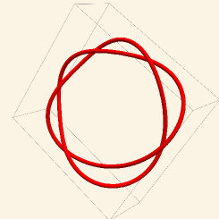
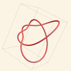
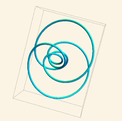
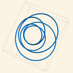
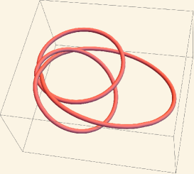
In the case (26a) we observe that the curve in \({\mathbb{R}}^{3}\) is a right-handed \((q,p+q)\) torus knot. Recall that the type of a \((m,n)\) torus knot depends only on the unordered pair \(\{m,n\}\). However, for our examples we find that when \(k\) is close to its lower limit, the knot takes a shape with \(q\) strands that wind along the torus the long way (see Figure 1, top left, where \(k=-3.85\gtrsim-4\)), while when \(k\) is close to its upper limit the knot has \(p+q\) strands winding the long way (see Figure 1, bottom right, where \(k=0.2\lesssim 0.5.\)) In general, the knot shape is more compact and symmetric when \(\lambda=0\); Figure 2 shows two shapes for the same \(p,q,k\) but different \(\lambda\) values. Note that (25) shows that these curves have the same differential invariant \(z\) but different constant values \(m=b\).
We showed in Lemma 12 of [3] that transverse curves for which \(z=0\) identically are \(SU(2,1)\)-congruent to curves which run along the circular fibers of the Hopf fibration. Thus, when \(k\) approaches one of the roots \(m_{j}\), \(a=|z|\) will approach zero and the closed curve will approach a multiply-covered circle congruent to a Hopf fiber. In Figure 1, we show a family of right-handed \((2,5)\) torus knots, corresponding to a range of \(k\)-values, where at both ends of the family the curve approaches a multiply-covered circle.
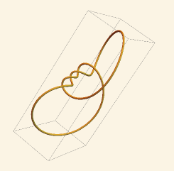
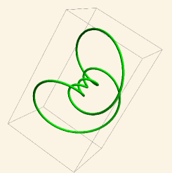
In the case (26b) we observe that the curve in \({\mathbb{R}}^{3}\) is a left-handed \((p,q)\) torus knot. (When \(p=1\) or \(q=1\) the curve is unknotted, as shown in Figure 4.) When \(k\) is close to its lower limit the curve has \(p\) strands winding around the torus the long way, and its shape approaches a circle covered \(p\) times. For large values of \(k\), the curve approaches a flattened teardrop shape, with the knot crossings compressed into a small region near where \(x=\pi\). Both these limiting behaviors are illustrated in Figure 3.


4.4 Constructing Transverse Curves
Once we have a fundamental matrix solution \(\Phi\) for the linear system (13), the first component of the \(\lambda\)-natural frame is then given by
| \(\Gamma=F\mathsf{e}_{1}=\Phi^{\dagger}\mathsf{e}_{1},\) |
taking value in the null cone \(\mathcal{N}\). We produce curves in \(S^{3}\) using a projection \(\hat{\pi}:\mathcal{N}\to S^{3}\) given in terms of the components of \(\Gamma\) by
| \(z_{1}=\dfrac{\Gamma_{3}-\mathrm{i}\Gamma_{1}}{\Gamma_{3}+\mathrm{i}\Gamma_{1}}% ,\qquad z_{2}=\dfrac{\sqrt{2}\,\Gamma_{2}}{\Gamma_{3}+\mathrm{i}\Gamma_{1}},\) | (30) |
where \((z_{1},z_{2})\) lie on the unit sphere in \({\mathbb{C}}^{2}\) equipped with its standard Hermitian inner product. For purposes of visualization, we in turn apply stereographic projection into \({\mathbb{R}}^{3}\) (using the point \(z_{1}=0\), \(z_{2}=\mathrm{i}\) as pole) given by
| \(\sigma:(z_{1},z_{2})\mapsto\left(\dfrac{\operatorname{Re}z_{1}}{1-% \operatorname{Im}z_{2}},\dfrac{\operatorname{Im}z_{1}}{1-\operatorname{Im}z_{2% }},\dfrac{\operatorname{Re}z_{2}}{1-\operatorname{Im}z_{2}}\right).\) |
Remark.
The action of \(SU(2,1)\) on the null cone preserves the 1-form \(\alpha_{N}=(dg,g)\), which is the pullback under \(\hat{\pi}\) of the standard contact form on \(S^{3}\), given by \(\alpha_{S}=\tfrac{1}{2}\operatorname{Im}(\overline{z}_{1}dz_{1}+\overline{z}_{% 2}dz_{2})\). The contact planes in \(S^{3}\) annihilated by this 1-form are orthogonal to the Hopf fibers. Since \(S^{3}\) is parallelizable, we can choose an globally defined orthogonal frame \((\mathsf{v}_{0},\mathsf{v}_{1},\mathsf{v}_{2})\) such that \(\mathsf{v}_{1},\mathsf{v}_{2}\) are tangent to the contact planes. For purposes of visualizing the contact distribution, we will use the following vectors in \({\mathbb{R}}^{3}\) which are tangent to the image of this distribution under stereographic projection:
| \(\displaystyle\sigma_{*}\mathsf{v}_{1}\) | \(\displaystyle=-(z+xy)\dfrac{\partial}{\partial{x}}+\tfrac{1}{2}(x^{2}-y^{2}+z^% {2}-1)\dfrac{\partial}{\partial{y}}+(x-yz)\dfrac{\partial}{\partial{z}},\) | ||
| \(\displaystyle\sigma_{*}\mathsf{v}_{2}\) | \(\displaystyle=\tfrac{1}{2}(x^{2}-y^{2}-z^{2}+1)\dfrac{\partial}{\partial{x}}+(% xy-z)\dfrac{\partial}{\partial{y}}+(xz+y)\dfrac{\partial}{\partial{z}}.\) |
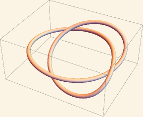
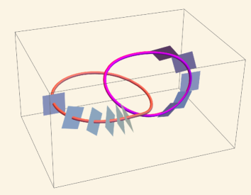
Figure 4 shows how the curve \(\gamma\) is transverse to the planes spanned by these vector fields.
Recall from (6) that when \(m=0\) the frame vector \(V\) projects to a Legendrian curve in \(S^{3}\). Figure 4 also shows this companion curve which in this example is linked with \(\gamma\) and tangent to the contact planes.
5 Discussion
We have shown how the YO equations arise, somewhat unexpectedly, from a simple geometric flow for curves in \(S^{3}\) that are transverse to the standard contact structure. The recent renewed interest in the YO equations and related systems (see, e.g., [4, 5, 8]), the analogies between the geometric flow considered in this work and the vortex filament flow, and the relatively simple reconstruction of the transverse curve in terms of solutions of the YO Lax pair, makes this a good case for exploring questions such as recursion schemes and the geometric and topological properties of transverse curves related to special solutions of the YO equations.
A natural direction of investigation is the study of the integrable hierarchy of vector fields for transverse curves associated with the YO hierarchy. These are generated by beginning with a conserved density for the YO equations, e.g.,
| \(\rho_{1}=\tfrac{1}{2}m,\quad\rho_{2}=\tfrac{1}{2}|z|^{2},\quad\rho_{3}=\tfrac{% 1}{2}\operatorname{Im}(\overline{z}z_{x})-\tfrac{1}{8}m^{2},\quad\rho_{4}=-% \tfrac{1}{2}\left(m|z|^{2}+|z_{x}|^{2}\right),\ldots\) |
and forming the vector field \(X_{n}=f_{n}\Gamma+g_{n}B+h_{n}V\) where \((\Gamma,B,V)\) is a natural frame. The coefficients are determined by the corresponding density as follows. As in (10) write \(z=k+\mathrm{i}\ell\) and express the density \(\rho_{n}\) in terms of real invariants \(k,\ell,m\) and their \(x\)-derivatives. Let
| \((a_{n},b_{n},c_{n})^{T}={\mathsf{E}}\rho_{n}\) |
where \(\mathsf{E}\) denotes the vector-valued Euler operator. Then the components of \(X_{n}\) are \(h_{n}=2c_{n}\), \(g_{n}=\mathrm{i}(a_{n}+\mathrm{i}b_{n})\) and \(f_{n}=-(c_{n})_{x}+\mathrm{i}d_{n}\), where \(d_{n}=\int\operatorname{Re}(g_{n}\overline{z})\;dx\). (Thus, these vector fields satisfy the conditions in (9) to preserve the adapted frame.)
The first few vector fields generated this way are
| \(\begin{split}X_{1}&=V=\Gamma_{x},\\ X_{2}&=\mathrm{i}zB=\mathrm{i}(\Gamma_{xx}-m\Gamma),\\ X_{3}&=\left(\tfrac{1}{4}m_{x}+\tfrac{1}{2}\mathrm{i}|z|^{2}\right)\Gamma+z_{x% }B-\tfrac{1}{2}mV,\\ X_{4}&=\left(\tfrac{1}{2}|z|^{2}_{x}-\mathrm{i}\operatorname{Im}(\overline{z}z% _{x})\right)\Gamma+\mathrm{i}(z_{xx}-mz)B-|z|^{2}V.\end{split}\) |
The fact that the antiderivative \(d_{n}\) is always expressible in terms of \(z,m\) and their derivatives is somewhat mysterious. However, we observe that these antiderivatives are expressible in terms of Hermitian inner products of the vector fields themselves:
| \(d_{2j}=-\tfrac{1}{2}\sum_{k=1}^{2j-2}\langle X_{2j-k},X_{1+k}\rangle,\qquad d_% {2j+1}=-\tfrac{1}{2}\sum_{k=1}^{2j-1}(-1)^{k}\langle X_{2j+1-k},X_{1+k}\rangle.\) |
Since \(d_{n}=\operatorname{Re}\langle X_{n},V\rangle=\tfrac{1}{2}(\langle X_{n},V% \rangle+\langle V,X_{n}\rangle)\) and \(V=X_{1}\), these identities are equivalent to
| \(\sum_{k=0}^{2j-1}\langle X_{2j-k},X_{1+k}\rangle=0\qquad\text{and}\qquad\sum_{% k=0}^{2j}(-1)^{k}\langle X_{2j+1-k},X_{1+k}\rangle=0.\) |
These show a remarkable parallel with the situation for vector fields in the hierarchy for the vortex filament flow [10], where the antiderivative required for the tangential component of \(X_{n+1}\) is expressible in terms of inner products of the vector fields up to \(X_{n}\). In that case, the analogous identities were proved using the first-order ‘geometric’ recursion operator for the vector fields. In our case, it may be sufficient to have a second-order recursion operator that relates \(X_{n+2}\) to \(X_{n}\).
Bäcklund and Darboux transformations as well as Miura transformations are other common features of integrable systems. In particular, the classical Bäcklund transformation for the sine-Gordon equation has its origins in relating pair of pseudospherical surfaces through line congruences (see, e.g., §7.5 in [9]). It is possible that an analogous transformation exists between T-curves evolving by the YO flow (11); one might expect that the curves would be joined by a congruence of circles in \(S^{3}\) expressed in terms of the vectors of the natural frame.
In relation to a possible Miura transformation, one can investigate the evolution equations induced by (11) for the tangent indicatrix, i.e., the curve in \(S^{3}\) traced out by the projectivization of the frame vector \(V\). It is natural to ask how the invariants of these indicatrices are related to those of the primary curve, and furthermore whether, when the primary curve evolves by an integrable geometric flow, the invariants of the indicatrix evolve by a related integrable system.
Acknowledgments
We thank Emilio Musso for many fruitful discussions.
References
- [1]
- [2] R. L. Bishop, There is more than one way to frame a curve, American Math. Monthly, 822:46–51, 1975.
- [3] A. Calini, T. Ivey, Integrable geometric flows for curves in pseudoconformal \(S^{3}\), Journal of Geometry and Physics, 166, 104249, 2021.
- [4] M. Caso-Huerta, A. Degasperis, S. Lombardo, M. Sommacal, A new integrable model of long wave–short wave interaction and linear stability spectra, Proc. R. Soc. A. 477 (2021) 20210408.
- [5] M. Caso-Huerta, A. Degasperis, S. Lombardo, M. Sommacal, Periodic and solitary wave solutions of the long wave– short wave Yajima-Oikawa-Newell model, Fluids 7 (7) (2022) 227.
- [6] V. Djordjevic, L. Redekopp, On two-dimensional packets of capillary-gravity waves, Journal of Fluid Mechanics, 79(4), 703-714, 1977.
- [7] R.H.J. Grimshaw, The modulation and stability of an internal gravity wave, Res. Rep. School Math. Sci., Univ. Melbourne, no. 32, 1975.
- [8] R. Li, X. Geng, Periodic-background solutions for the Yajima–Oikawa long-wave–short-wave equation, Nonlinear Dyn. 109 (2) (2022) 1053–1067.
- [9] T.A. Ivey, J.M. Landsberg, Cartan for Beginners: Differential Geometry via Moving Frames and Exterior Differential Systems (2nd ed.), Graduate Studies in Mathematics 175, American Mathematical Society, 2016
- [10] J. Langer, Recursion in Curve Geometry, New York J. Math. 5, 25–51 (1991).
- [11] J. Langer, R. Perline, Poisson geometry of the filament equation, J Nonlinear Sci 1, 71–93 (1991).
- [12] O. C. Wright, Homoclinic Connections of Unstable Plane Waves of the Long-Wave–Short-Wave Equations, Studies in Applied Mathematics 117:71–93, 2006.
- [13] N. Yajima, M. Oikawa, Formation and Interaction of Sonic-Langmuir Solitons, Progress of Theoretical Physics, 56(6), 1719–1739, 1976.
- ×
- × R. L. Bishop, There is more than one way to frame a curve, American Math. Monthly, 822:46–51, 1975.
- × A. Calini, T. Ivey, Integrable geometric flows for curves in pseudoconformal \(S^{3}\), Journal of Geometry and Physics, 166, 104249, 2021.
- × M. Caso-Huerta, A. Degasperis, S. Lombardo, M. Sommacal, A new integrable model of long wave–short wave interaction and linear stability spectra, Proc. R. Soc. A. 477 (2021) 20210408.
- × M. Caso-Huerta, A. Degasperis, S. Lombardo, M. Sommacal, Periodic and solitary wave solutions of the long wave– short wave Yajima-Oikawa-Newell model, Fluids 7 (7) (2022) 227.
- × V. Djordjevic, L. Redekopp, On two-dimensional packets of capillary-gravity waves, Journal of Fluid Mechanics, 79(4), 703-714, 1977.
- × R.H.J. Grimshaw, The modulation and stability of an internal gravity wave, Res. Rep. School Math. Sci., Univ. Melbourne, no. 32, 1975.
- × R. Li, X. Geng, Periodic-background solutions for the Yajima–Oikawa long-wave–short-wave equation, Nonlinear Dyn. 109 (2) (2022) 1053–1067.
- × T.A. Ivey, J.M. Landsberg, Cartan for Beginners: Differential Geometry via Moving Frames and Exterior Differential Systems (2nd ed.), Graduate Studies in Mathematics 175, American Mathematical Society, 2016
- × J. Langer, Recursion in Curve Geometry, New York J. Math. 5, 25–51 (1991).
- × J. Langer, R. Perline, Poisson geometry of the filament equation, J Nonlinear Sci 1, 71–93 (1991).
- × O. C. Wright, Homoclinic Connections of Unstable Plane Waves of the Long-Wave–Short-Wave Equations, Studies in Applied Mathematics 117:71–93, 2006.
- × N. Yajima, M. Oikawa, Formation and Interaction of Sonic-Langmuir Solitons, Progress of Theoretical Physics, 56(6), 1719–1739, 1976.
Contents
- 1 Introduction
- 2 Pseudoconformal Frames and Curvature
- 3 Curve Flows and the Yajima-Oikawa Equations
-
4 Plane wave solutions
- 4.1 Equivalent Versions of YO
- 4.2 Wright’s Solutions
- 4.3 Visualizing Examples
- 4.4 Constructing Transverse Curves
- 5 Discussion