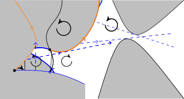
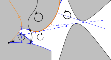
2.4.2 Root trails and connected components of the minimal set
2.5 Asymptotic geometry of Hutchinson invariant sets
2.5.1
2.5.2
3 Local analysis of the boundary of
3.1 Description of a tangent cone
3.2 Curve of inflections
3.2.1 Inflection domains
3.2.2 Circle at infinity
3.2.3 Singularities of the vector field
3.2.4 Tangency locus
3.3 Horns
3.3.1 Definitions
3.3.2 Small horns exist
3.3.3 Removing small horns
4 Boundary arcs
4.1 The correspondences and
4.2 Support lines
4.3 Local arcs
4.4 Local connectedness of
4.5 Global arcs
4.5.1 Additional results about correspondence
4.5.2 Orientation of global arcs
4.6 Points of extruding type
4.7 Boundary arcs in inflection domains
5 Singular boundary points on the curve of inflections
5.1 Horns at points of the transverse locus
5.2 Points of bouncing type
5.3 Points of -inflection type
5.4 Points of -inflection type
5.5 Points of switch type
5.6 Classification of boundary points
5.7 Estimates concerning local and global arcs
5.8 Long arcs
5.8.1 Estimates concerning long arcs
5.8.2 Admissible long arcs
5.8.3 Bounding the number of transverse intersection points between and the transverse locus of
6 Global geometry of minimal sets
6.1 Local convexity of the boundary
6.2 Case
6.2.1 Horizontal locus and special line
6.2.2 Asymptotic geometry of the minimal set
6.2.3 Examples
6.3 Case
6.4 Connected components of minimal sets
6.5 Case
6.5.1
6.5.2
6.5.3 The first family of examples
6.5.4 A second family of examples
On boundary points of minimal continuously Hutchinson invariant sets
Per Alexandersson
Department of Mathematics, Stockholm University, SE-106 91 Stockholm,
Sweden
per.w.alexandersson@gmail.com, Nils Hemmingsson
Institute for Mathematical Sciences, Stony Brook University, Stony Brook, NY, USA
nils.hemmingsson@stonybrook.edu, Dmitry Novikov
Faculty of Mathematics and Computer Science, Weizmann Institute of Science, Rehovot, 7610001 Israel
dmitry.novikov@weizmann.ac.il, Boris Shapiro
Department of Mathematics, Stockholm University, SE-106 91
Stockholm, Sweden
shapiro@math.su.se and Guillaume Tahar
Beijing Institute of Mathematical Sciences and Applications, Huairou District, Beijing, China
guillaume.tahar@bimsa.cn
(Date: March 2, 2026)
Abstact.
A linear differential operator with polynomial coefficients defines a continuous family of Hutchinson operators when acting on the space of positive powers of linear forms. In this context, has a unique minimal Hutchinson-invariant set in the complex plane. Using a geometric interpretation of its boundary in terms of envelops of certain families of rays, we subdivide this boundary into local and global arcs (the former being portions of integral curves of the rational vector field ), and singular points of different types which we classify below.
The latter decomposition of the boundary of is largely determined by its intersection with the plane algebraic curve formed by the inflection points of trajectories of the field . We provide an upper bound for the number of local arcs in terms of degrees of and . As an application of our classification, we obtain a number of global geometric properties of minimal Hutchinson-invariant sets.
Key words and phrases:
Action of linear differential operators,
-invariant subsets, minimal -invariant subset, rational vector fields
2020 Mathematics Subject Classification:
Primary 37F10, 37E35; Secondary 34C05
Contents
1 Introduction
1.1 Main results
1.2 Organization of the paper
2 Preliminary results and basic properties of
2.1 Regularity of the minimal set
2.2 Extended complex plane
2.3 Integral curves
2.4 Root trails
2.4.1 Concavity of root trails
2.4.2 Root trails and connected components of the minimal set
2.5 Asymptotic geometry of Hutchinson invariant sets
2.5.1
2.5.2
3 Local analysis of the boundary of
3.1 Description of a tangent cone
3.2 Curve of inflections
3.2.1 Inflection domains
3.2.2 Circle at infinity
3.2.3 Singularities of the vector field
3.2.4 Tangency locus
3.3 Horns
3.3.1 Definitions
3.3.2 Small horns exist
3.3.3 Removing small horns
4 Boundary arcs
4.1 The correspondences and
4.2 Support lines
4.3 Local arcs
4.4 Local connectedness of
4.5 Global arcs
4.5.1 Additional results about correspondence
4.5.2 Orientation of global arcs
4.6 Points of extruding type
4.7 Boundary arcs in inflection domains
5 Singular boundary points on the curve of inflections
5.1 Horns at points of the transverse locus
5.2 Points of bouncing type
5.3 Points of -inflection type
5.4 Points of -inflection type
5.5 Points of switch type
5.6 Classification of boundary points
5.7 Estimates concerning local and global arcs
5.8 Long arcs
5.8.1 Estimates concerning long arcs
5.8.2 Admissible long arcs
5.8.3 Bounding the number of transverse intersection points between and the transverse locus of
6 Global geometry of minimal sets
6.1 Local convexity of the boundary
6.2 Case
6.2.1 Horizontal locus and special line
6.2.2 Asymptotic geometry of the minimal set
6.2.3 Examples
6.3 Case
6.4 Connected components of minimal sets
6.5 Case
6.5.1
6.5.2
6.5.3 The first family of examples
6.5.4 A second family of examples
1 Introduction
Given a linear differential operator
(1.1)
where are polynomials that are not identically vanishing, we say that a closed subset is continuously Hutchinson invariant for (-invariant set for short) if for any and any arbitrary non-negative
number , the image of the function either has all roots in or vanishes identically. In [AHN+24], we have initiated the study of general topological properties of -invariant sets.
The main motivation for the present study that it covers an interesting and manageable special case of a more general inverse Pólya-Schur problem introduced in [ABS]. For the convenience of our readers, let us briefly recall what the Pólya–Schur problem/theory and its inverse are, see [CsCr, ABS].
The main question of the classical Pólya–Schur theory
can be formulated as follows.
Problem 1.1.
Given a subset of the complex plane, describe the
semigroup of all linear operators
sending any polynomial with roots in to a
polynomial with roots in (or to ).
Definition 1.2.
If an operator has the latter property, then we say that
is a -invariant set, or that preserves .
So far 1.1 has only been solved for the circular domains (i.e., images of
the unit disk under Möbius transformations), their boundaries [BB],
and more recently for strips [BCh]. Even a very similar case of the unit interval is still open at present. It seems that for a somewhat general class of subsets , 1.1 is currently out of reach of all existing methods.
In [ABS], the following inverse problem in the Pólya–Schur theory which seems both natural and more accessible than Problem 1.1 has been proposed.
Problem 1.3.
Given a linear operator , characterize all closed -invariant subsets of the complex plane. Alternatively, find a sufficiently large class of
-invariant sets.
Paper [ABS] concentrates on the fundamental case when is a linear finite order differential operator with polynomial coefficients and shows that under some weak assumptions on these coefficients, there exists a unique minimal -invariant set (and its analogs when acts on polynomials of degree greater than or equal to a given positive integer ). Many basic properties of -invariant sets such as their convexity, compactness etc are discussed in [ABS] as well as the delicate connection of Problem 1.3 to the classical complex dynamics.
However effective criteria characterizing -invariant sets and explicit description of the minimal -invariant set in somewhat interesting cases are currently missing which motivated the consideration in [AHN+24] of the action of on integer and positive powers of linear forms. This situation is still quite interesting and appears to be more tractable.
In particular, the following results have been obtained in [AHN+24]:
•
provided that either or is not a constant polynomial, there is a unique minimal continuously Hutchinson invariant set for a given operator (in what follows we will always assume that this condition is satisfied);
•
the only -invariant set is the whole unless ;
•
a complete characterization of operators for which has an empty interior has been obtained (see Section 2.1 for details).
In this paper, we will focus on operators whose minimal set has a nonempty interior.
Definition 1.4.
For an operator given by (1.1) with and not vanishing identically, at each point such that , we define the associated ray as the half-line .
Remarkably, -invariant sets (and, in particular, the minimal one) can be characterized in terms of associated rays.
Theorem 1.5(Theorem 3.18 in [AHN+24]).
A closed subset is -invariant if and only if it satisfies the following two conditions:
(1)
contains the roots of the polynomials and ;
(2)
for any point , the associated ray is disjoint from .
1.1 Main results
In the present paper, using Theorem 1.5, we provide a qualitative description of the boundary of minimal continuously Hutchinson invariant sets, including an exhaustive typology of its singular points. Our classification mainly depends on the intersection of the boundary with the curve of inflections of the field .
Definition 1.6.
The curve of inflections of the vector field is defined as the closure of the set of points satisfying , see [AHN+24]. It is a real plane algebraic curve of degree at most (in this paper, we will always have ).
The curve of inflections splits the complex plane into inflection domains where the sign of remains the same.
Points of outside its intersection with are classified with the help of two correspondences and sending the boundary to itself and defined as follows:
For a given point of the boundary , is essentially the intersection of with the integral curve of the rational field starting at , where . In contrast, is the intersection of the associated ray with the closure of in the compactification of the complex plane (see Section 2.2). Formal definitions of and are given in Definition 4.1. Qualitatively, the boundary is made of two kinds of arcs:
•
local arcs which are integral curves of the field (i.e. and );
•
global arcs at each point of which the associated ray is tangent to elsewhere (i.e. and ).
Local arcs are locally strictly convex real-analytic arcs (see Proposition 4.11). In contrast, global arcs (formed by points of global type) can fail to be .
Local arcs inherit an obvious orientation from the vector field . Global arcs also have canonical orientation, but its definition requires some work (see Section 4.5.2).
Local and global arcs connect special singular points of which in most of the cases belong to the curve of inflections. The latter decomposes into three loci (singular, tangent and transverse), each determining its own variety of singular points.
Definition 1.7.
The curve of inflections of the field decomposes into:
•
the singular locus formed by the points where several branches of intersect;
•
the tangency locus formed by the non-singular points where the field is tangent to ;
•
transverse locus formed by the non-singular points of where the field is transverse to .
The singular and the tangency loci are given by algebraic conditions. Therefore their intersection with is controlled in terms of and . On the contrary, many points of the boundary can belong to the transverse locus . We refine the definition of the correspondence according to the value of (which, by definition, is a positive number).
Definition 1.8.
We define , where are closures of in the compactification of , respectively.
For any , we have where belongs to:
•
if ;
•
if ;
•
if ,
and belongs to
•
if ;
•
if ;
•
if .
In particular, if , then .
The main result of the present paper is a classification of boundary points of minimal continuously Hutchinson sets.
Theorem 1.9.
For any linear differential operator given by (1.1), any point of the boundary of its minimal -invariant set belongs to one of the following types:
•
roots of polynomials and (at most of them);
•
singular points of the curve of inflections (at most of them);
•
tangency points between the curve of inflections and the field :
–
straight segments, half-lines and lines (contained in at most lines);
–
at most isolated points;
•
points of the transverse locus belonging to one of the four subclasses:
–
bouncing type: and ;
–
switch type: and ;
–
-inflection type: , and ;
–
-inflection type: and either or .
•
points not on the curve of inflections belonging to one of the three subclasses:
–
local type: and ;
–
global type: and ;
–
extruding type: and .
Here, .
There can be many singular points of bouncing, extruding, -inflection, -inflection and switch types (we do not have a polynomial bound of their number in terms of and ). An extensive description of their geometric features is given below:
•
at points of extruding type, the boundary of is not convex and it switches from a global to a local arc (see Section 4.6 and Fig.1);
•
at points of bouncing type, hits the curve of inflections, but does not cross it. In a neighborhood of such a point, the boundary remains in the closure of the same inflection domain (see Section 5.2 and Fig.1);
•
at points of switch type, is strictly convex, crosses the curve of inflections and the boundary switches from a local to a global arc (see Section 5.5 and Fig.1);
•
at points of -inflection type, crosses the curve of inflections and it switches from a global to another global arc having the opposite orientation. At such a point the curvature of is discontinuous (see Section 5.4 and Fig.1);
•
at points of -inflection type, crosses the curve of inflections and the boundary switches from a global arc to a local arc. Besides, the curvature of is continuous at such a point (see Section 5.3 and Fig.1).
Figure 1. Top row from the left: Extruding type, Switch type. Bottom row from the left: -inflection type, -inflection type, Bouncing type. In the pictures, blue arcs are global arcs, red arcs are local arcs and the black arc is a germ of the curve of inflections. The pointed arrow is the associated ray indicating the support points, when applicable.
Our second main result is an upper bound on the number of points of -inflection, -inflection and switch type in terms of .
Theorem 1.10.
For any operator given by (1.1), the numbers of points of switch, -inflection and -inflection type (respectively , and ) in
satisfy the following bounds:
Corollary 1.11.
For any operator given by (1.1), the boundary of the minimal set contains at most local arcs.
In the last section of the paper, we deduce many results about the global geometry of minimal sets from the classification of boundary points. In several cases, an exact description can be given in terms of local and global arcs. In particular, we can prove that in generic case, the minimal -invariant set is connected in .
Theorem 1.12.
For any linear differential operator given by (1.1), the minimal continuously Hutchinson invariant set is a connected subset of with the possible exception of the case when is of the form with and .
In this later case, (unless both and are constants and then there is no reasonable notion of a minimal set), is formed by at most connected components.
1.2 Organization of the paper
•
In Section 2, we provide the basic background information on Hutchinson invariant sets developed in [AHN+24], including the results about their asymptotic geometry.
•
In Section 3, we describe the local geometry around singular points of the vector field in terms of their local degree and principal value. We also describe the main properties of the curve of inflections defined by the equation and we also introduce the notion of horns.
•
In Section 4, we describe boundary points in the complement to the curve of inflections, introducing and correspondences.
•
In Section 5, we classify boundary points in the generic locus of the curve of inflections, proving Theorems 1.9 and 1.10 (in Sections 5.6 and 5.8.3 respectively). Corollary 1.11 is also proved in Section 5.8.3.
•
In Section 6, we apply the latter results to get precise descriptions of minimal sets in several cases. Theorem 1.12 is proven in Section 6.4.
Acknowledgments. The third author is supported by the Israel Science Foundation (grants No. 1167/17 and 1347/23), by funding received from the MINERVA Stifting with the funds from the BMBF of the Federal Republic of Germany, and from the European Research Council (ERC) under the European Union Horizon 2020 research and innovation program (grant agreement No. 802107). The fourth author wants to acknowledge the financial support of his research provided by the Swedish Research Council grant 2021-04900 and the hospitality of the Weizmann institute of Science in April 2021 and January 2024 when substantial part of the project was carried out. He is sincerely grateful to Beijing Institute of Mathematical Sciences and Applications for the support of his sabbatical leave in the Fall of 2023. The fifth author would like to thank France Lerner for valuable remarks about the terminology related to singular points.
2 Preliminary results and basic properties of
The following notation will be important throughout this text.
Notation 2.1.
Given an operator as in (1.1), we define , and so that
Furthermore, we set and .
Similarly, for any point , we have with and . We denote by the argument of .
Remark 2.2.
Observe that frequently used affine changes of the variable are applied to the vector field and not to the rational function itself.
2.1 Regularity of the minimal set
For an operator as in (1.1), its minimal set can be of three possible types:
•
regular if coincides with the closure of its interior;
•
fully irregular if has empty interior;
•
partially irregular if has nonempty interior but is not regular.
Actually, irregularity is related to specific reality conditions. The characterization of operators for which is fully irregular is contained in Theorem 1.15 of [AHN+24].
Theorem 2.3.
For an operator as in (1.1), the minimal set is fully irregular in the following cases:
•
for some ;
•
for some , and ;
•
for some , and ;
•
operators satisfying the following conditions (up to an affine change of variable):
–
is real on ;
–
roots of and are real, simple and interlacing (i.e. the roots of and alternate along the real axis);
–
;
–
if , then .
In any other case, has a nonempty interior.
In this paper, we will always assume that has a nonempty interior.
Remark 2.4.
If , then is either totally irregular or coincides with (see Theorem 1.15 of [AHN+24]). Therefore, our operators will always satisfy . This implies in particular that satisfies .
Referring to the closure of the interior of as the regular locus and its complement in as the irregular locus, we observe that the latter is contained in very specific lines of the plane.
Definition 2.5.
For a given rational function , a line is called -invariant if for any such that is defined, we have .
In particular, up to an affine change of variable, we can assume and thus is a real rational function. Besides, a -invariant line is automatically an irreducible component of the curve of inflections .
Definition 2.6.
For an operator whose minimal set is not fully irregular, a tail is a semi-open straight segment in satisfying the following conditions:
•
the segment belongs to an -invariant line;
•
for any , ;
•
for any , is disjoint from the regular locus of ;
•
belongs to the regular locus of ;
•
;
•
is a root of the same multiplicity for both and .
In particular, every tail belongs to a -invariant line.
The following fact has been proven in Corollary 7.8 of [AHN+24].
Theorem 2.7.
For an operator whose minimal set is not fully irregular, the irregular locus of is a (possibly empty) finite union of tails.
In particular, if and have no common roots, then the minimal set of the corresponding operator is either regular or fully irregular.
2.2 Extended complex plane
Following Theorem 1.5, -invariant sets are characterized by the position of the associated rays starting in their complements. Let us introduce a certain compactification111Notice that the most frequently used compactification of is . of which comes very handy in our considerations. We baptise it the extended complex plane .
The extended complex plane is set-theoretically the disjoint union of and endowed with the topology defined by the following basis of neighborhoods:
•
for a point , we choose the usual open neighborhoods of in ;
•
for a direction , we choose open neighborhoods of the form where is an open interval of containing and is an open cone with apex whose opening (i.e. the interval of directions) is .
Definition 2.8.
Given as above, let be a non-singular point of . We define as the argument of . We think of as a point of the circle at infinity.
One can easily see that of the extended plane can be identified with the above circle at infinity. The extended plane is compact and homeomorphic to a closed disk. In particular, usual straight lines in have compact closures in . (Below we will make no distinction between a real line in and its closure in ). Open half-planes in are, by definition, connected components of the complement to a line.
Given a -invariant set , we denote by its closure in the extended plane .
The following result, but with a slightly different formulation, has been proved in Lemma 4.4 of [AHN+24].
Lemma 2.9.
Given an -invariant set , let be such that:
•
, ;
•
;
•
is homotopic to the positive arc from to in the circle at infinity via a homotopy such that for all .
If denotes the connected component of in containing the interval in the complement of , then .
2.3 Integral curves
Another result has been proved in Proposition A.2 of [AHN+24].
Proposition 2.10.
Given a -invariant set and some point , if there is a positively oriented integral curve of the vector field such that , then for any , .
When referring to the proposition above, we say that the bounded backward trajectories of of points in any invariant set belongs to .
2.4 Root trails
For any point , the root trail of is the closure of the set of points such that the associated ray contains . Except for the trivial cases described in Section 3 of [AHN+24], root trails are plane real-analytic curves. By definition, the root trail of any point of is also contained in . Furthermore, for any fixed , we defined a -trace (corresponding to ) as any continuous function such that
for all . That is, any -trace is a concatenation of parts of such that the resulting curve is continuous for any .
Lemma 2.11.
Consider a linear differential operator given by (1.1) and some point . Assuming that is not of the form ,
then
(i) for any point and any point such that and , the root trail has a unique branch passing through and its tangent slope is the argument of (mod ).
(ii) If and is the smallest integer such that , then has intersecting branches at . Their tangent slopes are:
where is the argument of and .
Before proving Lemma 2.11 we prove the next two Lemmas.
Lemma 2.12.
If is smooth planar curve, , and for some function holomorphic and non-vanishing at then the sign of the curvature of at coincides with the sign of .
Indeed, then . By definition, the sign of the curvature of at coincides with the sign of
.
Lemma 2.13.
Let be a function holomorphic at with and let . Then the germ of at consists of smooth branches with tangent slopes , , where .
If and is a parameterization of such that then the sign of the curvature of coincides with the sign of .
Proof.
Indeed, we have , , so the branches of are tangent to the lines satisfying equation , which have slopes as stated.
For the second claim, note that , so the claim follows from Lemma 2.12.
∎
Remark 2.14.
Similar results hold for having a pole at by considering .
Proof of Lemma 2.11.
Note that by definition
and Lemma 2.11 follows from the Lemma 2.13 with and the fact that .
∎
Remark 2.15.
The condition means that the point is obtained as the the first iteration of Newton’s method of approximating roots of with the starting point .
When is a point at infinity in the extended plane , the root trail of is the closure of the points where the argument of coincides with .
Lemma 2.16.
Consider a linear differential operator given by (1.1) such that is not constant. For any point at infinity and any point such that , provided , the root trail has a unique branch passing through and its tangent slope is the argument of (mod ).
If and is the smallest integer such that , then has intersecting branches at . Their tangent slopes are:
where is the argument of and .
Proof.
In this case and the claim follows again from Lemma 2.13
∎
Remark 2.17.
From Lemmas 2.11 and 2.16 it immediately follows that if a root trail can have branches at some point , then belongs to the curve of inflections (because and are real colinear).
Besides, if , then for and is a singular point of .
2.4.1. Concavity of root trails
Proposition 2.18.
Let be a point of the extended plane and be a point of such that and . We denote by the tangent line to at . We define to be:
•
if ;
•
if is a point at infinity.
Then the germ of at belongs to
(i) the same half-plane bounded by as the associated ray if and have opposite signs.
(ii)
They belong to distinct half-planes bounded by if and have the same sign.
Finally, has an inflection point at if .
Proof.
Let for and for so that . Let .
We have
If is a local parameterization of at such that then . Moreover, if the curvature of is positive and otherwise.
The tangent ray lies in if and in otherwise.
By Lemma 2.13 the sign of curvature of is opposite to the sign of .
For we have and
so we are interested in signs of
(recall that ) and
(2.1)
For we have and we are interested in the signs of
and .
∎
In the transverse locus of the curve of inflections, the concavity of root trails with respect to the line containing the associated ray depends on the sign of some geometrically meaningful real function.
Proposition 2.19.
Consider a point and some point . Assume that (or if is a point at infinity). Let be the line containing the associated ray .
The germ of at and the positive germ of the integral curve of the field starting at belong to the same open half-plane bounded by if is negative ( if is a point at infinity).
The germ of at and belong to opposite open half-planes bounded by if is positive ( if is a point at infinity).
Proof.
Without loss of generality, we assume that and with , and ( because belongs to the transverse locus of the curve of inflections). Necessarily . Since , belongs to the upper half-plane.
By Lemma 2.16, has a unique branch at tangent to .
Let for and for , so . Choose a parameterization of this branch in such a way that . Then
for or being a point at infinity, respectively.
Therefore if (resp. ) and otherwise.
By (2.1) the sign of the curvature of at is opposite to the sign of , i.e. is negative. Thus lies in the lower half-plane (i.e. not in the same half-plane as ) if is positive and in the same half-plane as if ( and resp. for ). Since , the number is invariant under the maps and used for normalization, and the claim follows.
∎
2.4.2. Root trails and connected components of the minimal set
When , root trails provide a bound on the number of connected components of the minimal set (in all other cases, it is known that is connected).
Proposition 2.20.
Consider a linear differential operator given by (1.1) and satisfying . Any connected component of satisfies the following conditions:
•
contains at least one root of ;
•
contains at least one root of ;
•
the sum of orders of zeros and poles of in vanishes.
Proof.
We assume that a connected component of is disjoint from . Note that implies that the union of the zeros of for any , and is bounded.
Hence, for any , the root trail of is disjoint from , as otherwise there would be points in the complement of belonging to the root trail of . Since coincides with the -extension of any point in (see Lemma 2.2 of [AHN+24]), it follows that cannot belong to the minimal invariant set.
Suppose now that there is a component for which the sums of orders of the zeros of does not equal the sums of orders of the zeros of . Then there is a component such that the sums of the orders of the zeros of , say is strictly greater than the sums of the orders of the zeros of , say . Taking we have that for all , the zeros of belonging to have total degree . However, when sending , of these zeros tend to the zeros of belonging to and at most one tend to . This implies that at least of the end points of the root trail of does not belong to , a contradiction.
∎
We prove now that the interior of the minimal set satisfies (outside zeroes and poles of ) a weak property of local connectedness.
Lemma 2.21.
For any linear differential operator given by (1.1) we consider a point of the boundary that is neither a zero nor a pole of . For any sufficiently small neighborhood of , the connected component of containing has connected interior.
Proof.
If does not belong to the regular locus of , then is a line segment and hence has empty interior.
We have for some . Then, a continuity argument immediately shows that has connected interior, as otherwise points in the complement of would have associated rays intersecting .
∎
In the following, we prove that the closure of a connected component of the interior of cannot be disjoint from .
Lemma 2.22.
For any linear differential operator given by (1.1), one of the following statements holds:
(1)
is fully irregular;
(2)
;
(3)
the closure of any connected component of the interior of the minimal set contains a root of ;
(4)
the closure of any connected component of the interior of the minimal set contains an endpoint of a tail.
Proof.
We suppose that we are not in the case (1), (2). Besides, we assume the existence of a connected component of the interior of the minimal set whose closure is disjoint from , contradicting statement (3).
We first prove that cannot be the only connected component of . Indeed, roots of that do not belong to the regular locus of (the closure of the interior) belong to tails (see Theorem 2.7) and they are not zeros or poles of . Besides, is assumed to be distinct from . Consequently, we have . The only case where the regular locus of can be disjoint from is when is of the form or . In the first case, is known to be totally irregular. In the second case, either (and is totally irregular, see Theorem 2.3) or and has no tails (and has no root at all). We assume therefore that the interior has several connected components.
We denote by the set of points of that belong to the closure of another connected component of . By assumption, these are not these points are not roots of and Lemma 2.21 shows that each of them is a zero of .
Since is minimal, there is a point and a point . As the root trail changes continuously in , may be chosen outside . Since , the zeros of as tends to . Further, we can assume that does not equal for some finite , as this would imply and , in which case is equal to . Hence, the minimal set therefore contains a continuous path from an element of to such that solves .
The path has to enter the component and can do so either through a tail or an element of . The path cannot contain any element because the equations and (for some ) imply , contradicting our assumption. Our assumption that neither (1), (2) nor (3) was satisfied thus implies (4).
∎
2.5 Asymptotic geometry of Hutchinson invariant sets
Let us recall the results of [AHN+24] concerning minimal Hutchinson invariant sets (see Theorems 1.11 and 1.12 of [AHN+24]).
Theorem 2.23.
For any operator as in (1.1) with a minimal set having a nonempty interior, is:
•
a compact contractible subset of if , and ;
•
a noncompact non-trivial subset of if or ;
•
trivial, i.e. equal to otherwise.
Besides, the closure in the extended plane is contractible, connected and compact.
Thus, the only interesting cases for the description of are those for which the values of are , or . In the latter two cases, we have more precise results given below.
2.5.1.
The following statement has been proved in Corollary 6.2 of [AHN+24].
Proposition 2.24.
For an operator as in (1.1) such that . Then the complement of its minimal Hutchinson invariant set in has exactly two connected components .
Each contains infinite cones whose intervals of directions are arbitrarily close to and respectively.
2.5.2.
The following statement has been proven in Corollary 6.4 of [AHN+24].
Proposition 2.25.
Take any operator as in (1.1) such that . Then for any , there exists an open cone whose interval of directions is arbitrary close to and such that is contained in .
3 Local analysis of the boundary of
We consider an operator as in (1.1) whose minimal set has a nonempty interior.
Notation 3.1.
For any point , we define , so that
(3.1)
We also define and where .
3.1 Description of a tangent cone
Definition 3.2.
For any , we define as the subset of formed by directions such that there is a sequence satisfying the following conditions:
•
for any , ;
•
;
•
.
We also define as the subset of formed by directions such that the half-line does not intersect the interior of .
Lemma 3.3.
For any , the following statements hold:
(1)
and are nonempty closed subsets of ;
(2)
;
(3)
for any , . In particular,
is invariant under ;
(4)
for any , there exists a closed interval of length at most containing both and ;
(5)
.
Proof.
From Definition 3.2 it immediately follows that and are closed subsets of .
If , then we can find a sequence of points in the complement of approaching . By compactness of , we can choose a subsequence for which the arguments converge to some limit. Thus is nonempty.
Then, for any , we have a sequence in the complement of accumulating to with the limit slope . The associated rays accumulate to . Since none of them intersects the interior of , the half-line does not intersect it either and .
Besides, in the case where , (up to taking a subsequence of , there is a closed interval such that:
•
the endpoints of are and ;
•
the length of is at most ;
•
for any in the interior of , there is a bound such that for any , the associated ray intersects the half-line at some point .
Existence of sequences proves that for any , one has .
Finally, because in this case, would have empty interior.
∎
Remark 3.4.
Note that in the case , the interval is a singleton
Let us deduce local description of and depending on the local invariants of .
Corollary 3.5.
For any , the following statements hold:
•
if , then and they are contained in the finite set of arguments satisfying ;
•
if , then and ;
•
if , then ;
•
if , then and these sets are formed by at most two intervals, each of length at most and having their midpoints at and .
Proof.
We consider maximal interval in (which is non-empty by Lemma 3.3). The images of under the iterated action of belong to .
If , then is a singleton since otherwise the union of its iterates would coincide with (contradicting Lemma 3.3). Thus has to be a fixed point of the map .
If and , then coincides with because no other connected subset of the circle is preserved under the action of nontrivial rotation. Therefore is the identity map.
If , then for any , . Therefore .
If , then is invariant under the action of . Thus, either or is the bisector of . If is of length strictly bigger than , then Lemma 3.3 shows that its complement (of length strictly smaller than ) is also contained in . Therefore which is a contradiction.
∎
We obtain a bound on the number of petals of that can be attached to a boundary point.
Corollary 3.6.
For any linear differential operator given by (1.1) we consider a point of the boundary . Then for any sufficiently small open subset the interior of the connected component of containing has at most:
•
connected components if ;
•
connected components if
where with and .
Proof.
If is not a zero or a pole of , then Lemma 2.21 proves the statement. Besides, if , Corollary 3.5 proves that is in the closure of at most components.
In the remaining cases, is a simple zero of . If is also a root of degree of , then it is a root of degree of .
We can divide and by while keeping the same minimal set (because in this case remains unchanged). Consequently, we can assume that is not a root of . Lemma 2.22 proves that for any connected component of such that is in the closure of , either some root of belongs to the closure of or some tail is attached to . If is in the closure of several connected components of , then a same root of cannot be in the closure of two of them because would fail to be contractible. Similarly a given tail is attached to only one connected component of (and contains at least one root of ). Therefore, is in the closure of at most components.
∎
3.2 Curve of inflections
In §A.3 of [AHN+24] we introduced the curve of inflections of an analytic vector field . By definition, it is the closure in of the subset of at each point of which the integral curve of the vector field passing through this point has zero curvature. Here and throughout, denotes the set of zeros of the function . Below we provide some additional information about .
For an operator for which is not of the form or for some and , the function is a non-constant rational function. Therefore the curve of inflections of (which is defined as the closure of the set of points for which ) is a real plane algebraic curve.
We first characterize the points at which several local branches of the curve of inflections intersect.
Lemma 3.7.
A point belongs to exactly local branches of in the following cases:
(1)
is a critical point of of order (including zeroes of order of );
(2)
is a pole of of order .
The limit slopes of the local branches at form a regular -gon in .
Proof.
This follows immediately from Lemma 2.13.
∎
Corollary 3.8.
The curve of inflections has at most singular points.
Proof.
There are at most poles of and the critical points of are the zeroes of .
∎
Lemma 3.9.
Let be a non-constant rational function of degree . Then the real algebraic curve is non-empty, has at most connected components and has exactly connected components for generic .
Proof.
Clearly, as for any , as well.
By the open mapping theorem, the map , where is the closure of in , is onto on each connected component of . Since has degree this means that has at most components.
Note that the ramification points of coincide with the ramification points of lying on . Thus if the ramification values of are not in then the former map is an unramified cover of degree , so has exactly connected components. This means that the bound is sharp.
∎
3.2.1. Inflection domains
Definition 3.10.
The curve of inflections subdivides into two open (not necessarily connected) domains:
given by and given by .
Observe that in (resp. ), the integral curves of the vector field are turning counterclockwise (resp. clockwise).
3.2.2. Circle at infinity
Consider the closure of the curve of inflections in the extended complex plane .
Lemma 3.11.
The intersection is:
•
is empty if and ;
•
coincides with the set if .
In the remaining two cases:
•
and ;
•
; or
•
the set consists of points forming a regular -gon for some satisfying .
Proof.
If , then has an expansion of the form near from which the characterization of the infinite branches of the real locus of follows by Lemma 2.13 applied to either or to depending on whether or (clearly both have the same real locus outside their poles).
If , then has an expansion for some and near . (The case when is constant is ruled out by the genericity assumptions). Therefore has an expansion . We conclude that has infinite branches whose limit directions form a regular -gon.
If , then has an expansion for some , , and . (The case when is a linear function is ruled out by the genericity assumptions). We obtain that is of the form . Consequently, unless is real, the curve of inflections is compact in . If is real, the infinite branches of are asymptotically the same as that of the real locus of . Therefore has infinite branches whose limit directions form a regular -gon.
In these last two cases, we have for some and .
The number is the ramification index of either (for ) or (for ) at infinity, thus cannot be bigger than the degree of . Therefore .
∎
3.2.3. Singularities of the vector field
Next we deduce from Corollary 3.5 a proof of the statement that any root of or belonging to automatically belongs to the curve of inflections.
Corollary 3.12.
Consider an operator as in (1.1) such that does not coincide with and has a nonempty interior. Let be a zero or a pole of such that . Then also belongs to the curve of inflections . Additionally, the number of local branches of at equals:
•
if is a pole of order ;
•
if is a zero of order ;
•
some integer if is a simple zero.
Proof.
The statement is proved by direct computation of in case of a pole or a zero of order . If is a simple zero of , then we have . If , then (see Corollary 3.5). Thus .
Unless is linear, is of the form for some and . Thus . Consequently, the number of local branches of the equation equals .
If , then (otherwise ) and (otherwise is totally irregular). It follows that is a non-vanishing constant and the curve of inflections is empty. In this case, does not contain any zero or pole of on the boundary of .
∎
3.2.4. Tangency locus
Definition 3.13.
For the rational vector field , the tangency locus is the subset of the curve of inflections where is tangent to some branch of .
Proposition 3.14.
For an operator as in (1.1), the tangency locus is the union of:
•
at most lines and;
•
at most points.
Proof.
For any point , an immediate computation involving the Taylor expansion of proves that belongs to the intersection of the curve of inflections (given by ) with a real plane algebraic curve given by the equation . Indeed, the tangent line to at some is given by the equation , and the associated ray direction is . The degrees of these two curves are respectively and . Therefore, Bézout’s theorem implies that contains at most such points and some irreducible components corresponding to the common factors of the two equations.
By definition of the tangency locus these irreducible components are the integral curves of contained in the curve of inflections. Such integral curves have identically vanishing curvature and therefore they are segments of straight lines. Therefore the relevant irreducible components are straight lines.
But intersects at most points by Lemma 3.11. Thus the number of the lines is at most .
∎
We deduce an estimate on the number of connected components of the transverse locus of the curve of inflections. Denote .
Corollary 3.15.
For an operator as in (1.1), the transverse locus of the curve of inflections is formed by at most connected components.
Proof.
A connected component of is either a smooth closed loop (so a connected component of ) or an arc joining points at infinity, singular points of or isolated points of the tangency locus.
Following Proposition 3.14, the tangent locus contains at most isolated points. Each of them is the endpoint of two arcs of the transverse locus.
Lemma 3.11 proves that at most arcs of the transverse locus go to infinity.
Lemma 3.7 provides the analog result for the multiple points of the curve of inflections. In the ”worst” case, poles of and critical points of are simple. At most four arcs of the transverse locus are incident to such points. There are at most such points (see Corollary 3.8) so they are incident to at most arcs.
Adding these bounds, we obtain an upper bound on the number of ends of non-compact connected components of the transverse locus, i.e. there are at most non-compact connected components. By Lemma 3.9 the number of the compact connected components (loops) of is at most , which gives the required upper bound.
∎
Corollary 3.16.
On each connected component of the transverse locus , the sign of remains constant. If is positive (resp. negative), then for any point of the component, the associated ray points towards (resp. ).
Proof.
Any regular point of the curve of inflections satisfying belongs to the tangency locus (see the proof of Proposition 3.14). A direct computation proves the rest of the claim.
∎
3.3 Horns
In this section, we introduce some curvilinear triangles called horns and find conditions under which we can conclude that they do not belong to the minimal set . Our aim is to prove that some parts of the boundary of the minimal sets are portions of integral curves of the vector field .
3.3.1. Definitions
Recall that is the argument of , i.e. and is the associated ray.
Definition 3.17.
Assume that a segment of the positive trajectory of starting at and ending at doesn’t intersect the curve of inflections except possibly at . Assume that the total variation of along is less than .
We define the horn at as an open curvilinear triangle formed by and tangents to this trajectory at and intersecting at a point .
Definition 3.18.
A horn is called small positive (resp. small negative) if
(1)
for any point , the argument is monotone increasing (resp. decreasing) in the variable as long as and
(2)
for any two points , the scalar product is positive.
A horn is called small if it is either small positive or small negative.
Remark 3.19.
A small positive horn becomes a small negative one after conjugation, i.e. after replacing with . Indeed,
remains the same after the conjugation, and
changes sign.
Lemma 3.20.
The curve of inflections (given by ) does not intersect small horns.
Proof.
We have that . Assume that we have the equality at some . Since is open and is an open map, this assumption will imply that changes sign in , which contradicts the smallness assumptions.
∎
We define the cone complementary to (in short, the complementary cone) to be the open cone with the apex bounded by part of the ray starting at and by the ray extending the segment .
Lemma 3.21.
Consider a point which neither belongs to nor to the interior of . Assume that the integral curve of the vector field containing is not a straight line. Then there exists a horn such that both and its complementary cone do not intersect .
Proof.
Let .
First, assume that . Then by definition, .
Choose some and define and
(we stop when ).
The broken line is the Euler approximation to the positive trajectory of starting from and converges to it (more exact, to the connected component of containing ) as . Thus
Repeating this argument for all sufficiently close to we see that
(3.2)
If is a subset of the curve of inflections then it is a part of a straight line, which is excluded by our assumption. Thus we can assume that for sufficiently close to the curve intersects the curve of inflections only at . Therefore is convex and, choosing closer to if needed, we can assume that is of angle smaller than . Therefore
(3.3)
Second, assume that and let be a part of the connected piece of containing such that is convex and of angle smaller than . Let be a sequence of points tending to and take such that converges to . By analyticity this convergence is uniform in sense as well. Therefore
(3.4)
which finishes the proof.
∎
3.3.2. Small horns exist
Proposition 3.22.
For any point such that the trajectory of starting at is not a straight line, there exists a small horn .
Proof.
Using an affine change of variables we can assume that and . By assumption is not a real rational function.
Let
(3.5)
be the Taylor expansion of at (the case is covered by Lemma 3.23). Here we can assume that by replacing by , if necessary.
First, we consider the case , i.e. .
Lemma 3.23.
For every compact set not intersecting the curve of inflections , there is a such that for every , there is a small horn of diameter greater than .
Proof.
Indeed, for any the function is positive and are is non-zero at , so this remains true for all such that by continuity.
This means that any is a small horn. The uniform lower bound follows from the continuity of . ∎
From now on we assume that . Our next goal is to find the asymptotics of near and the . We abuse notation by writing the germ of as .
Lemma 3.24.
(3.6)
and
(3.7)
Proof.
Note that
(3.8)
Indeed,
Now,
(3.9)
so
For we get
Recalling that is tangent to the real axis, we have .
Therefore
near the origin, and the claim of the Lemma follows since .
∎
Next, we have to check the two conditions in Definition 3.18 for with sufficiently close to 0. The second condition is easy:
since then the scalar product is positive for all by continuity.
To check the first condition set with . By the second property of the small horns, we have . By (3.7) we have . Combining (3.9) and
(3.10)
we get
Thus, using (3.5), we get for the equation
(3.11)
where we use . This proves the first requirement of Definition 3.18.
∎
Corollary 3.25.
The germ of at cannot lie between and .
Proof.
This would mean that this germ lies inside which is impossible by Proposition 3.22 and Lemma 3.20.
∎
3.3.3. Removing small horns
We will use the following general Lemma
Lemma 3.26.
Assume that for some open set and every point , the associated ray lies in the union . Then .
Proof.
Indeed, if not then will be again invariant, which contradicts minimality of .
∎
The crucial property of small horns is the following Lemma.
Lemma 3.27.
For any , one has .
Proof.
We prove the statement assuming that the small horn is positive,
the negative case will follow by conjugation.
Figure 2. Removing small horns.
Let be a point such that . By definition of small horns, we have , see Fig. 2.
The ray does not intersect . Indeed, assume that the ray intersects at a point . Then at the intersection point the slope of should be smaller than the slope of , i.e. which contradicts the requirement that the slope is monotone increasing along the segment joining and .
Also cannot intersect since and , where such that .
Thus leaves and enters at some point of with the slope . Thus never leaves .
∎
Proposition 3.28.
Assume that is a small horn and .
Then is not in the interior of .
Proof.
Follows from Lemmas 3.26 and 3.27.
∎
4 Boundary arcs
Recall that we consider an operator whose minimal set is different from and has a nonempty interior. We want to describe its boundary in combinatorial and dynamical terms. To do this, we introduce two set-valued functions.
Recall that in our terminology, is the closure of in the extended plane .
4.1 The correspondences and
Definition 4.1.
For any , we define:
•
where is the positive trajectory of the vector field starting at ;
•
.
Note that if or , and then as well.
Using correspondences and , we split the set of boundary points of disjoint from the curve of inflections into the following three types.
Definition 4.2.
A point of is a point of:
•
local type if and ;
•
global type if and ;
•
extruding type if and .
By Proposition 4.7 these are the only possibilities for points in .
4.2 Support lines
In this (sub)section We prove that for a given point , the condition means that the associated ray is a support line of .
For any oriented support line of , we define the co-orientation of its support in the following way. The support point is:
•
a direct support point if the standard orientation of and the orientation of the support line agree at ;
•
an indirect support point otherwise.
In particular, if the support line is the positively oriented real axis, a support point is called direct if the intersection of with a neighborhood of is contained in the upper half-plane (see Figure 3 for examples of indirect support points).
Definition 4.3.
Consider such that:
•
does not belong to the tangency locus of the curve of inflections ;
•
is not a root of or .
Then we say that (resp. ) if the associated ray is pointing inside the inflection domain (resp. ). This includes (resp. ).
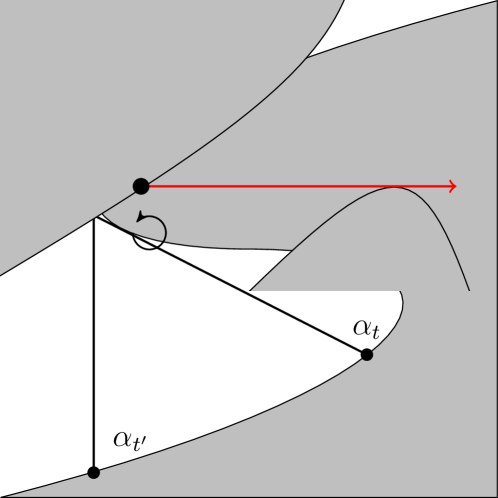
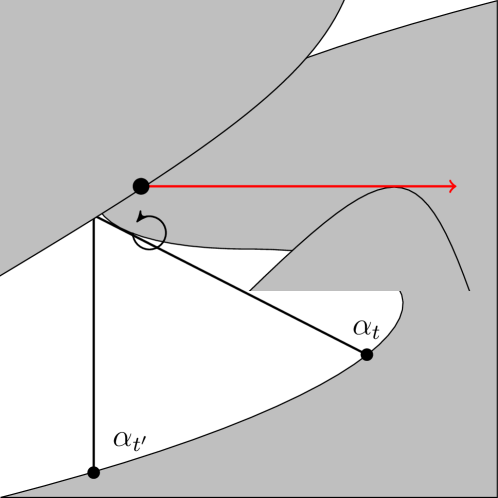
Figure 3. The point where the red arrow is tangent to is an indirect support point. The circular arrow indicates that the black point belongs to .
Lemma 4.4.
Consider such that (resp. ). If , then is an indirect support point (resp. a direct support point).
Proof.
Without loss of generality, we can assume that , , and .
This implies that lies in the upper half-plane. By Lemma 3.21 there is a neighborhood of such that is contained in the lower half-plane. Therefore is an indirect support point.
∎
Lemma 4.5.
Take such that:
•
•
the associated rays and intersect at some point ;
•
.
Then the open cone with apex and the interval of directions is disjoint from and there are the following subcases:
•
either or ;
•
either or .
Proof.
The path formed by the concatenation of segments and can be approached by a family paths joining and or a family of paths joining and whose interior points are disjoint from . Lemma 2.9 applies to one of these families of paths so is disjoint from .
Then, we assume by contradiction that and some point does not belong to . Since is disjoint from , it follows that is an indirect support point of the line containing which contradicts Lemma 4.4. Consequently either or .
An analogous argument proves that either or .
∎
4.3 Local arcs
In this section, we prove that local points (see Proposition 4.7)
form local arcs.
Definition 4.6.
A local arc of is a maximal open arc of an integral curve of vector field that contains only local points. In particular, it is disjoint from and .
Local arcs are oriented by the vector field .
Using the geometry of horns (see Section 3.3), we can show that every local point actually belongs to a local arc of .
Proposition 4.7.
Consider a point and such that and . Then, the germ of the integral curve of passing through belongs to .
Without loss of generality, we assume that , and , so lies in the upper half-plane. The proof consists of two steps illustrated by Figure 4 and Figure 5 respectively.
Lemma 4.8.
lies above the integral curve of passing through .
Proof: see Fig. 4.
By Lemma 3.21 there exists such that the union is outside of .
Let , , and let be the intersection point of with the line tangent to at . By Proposition 3.22 we can assume that
is a small horn at , . Clearly, .
The condition implies that . Moreover, as , there is an open sector with vertex on , containing and disjoint from .
For a point sufficiently close to and lying below consider a horn with vertices and close to and , respectively. By continuity, the part of starting from lies in . Also, lies in the horn , so by Lemma 3.21.
Thus the complementary cone of with vertex lies outside of . Therefore by Proposition 3.28 , so . As this remains true for any point in a sufficiently small neighborhood of , we conclude . Thus near the set lies above .
Figure 4. lies above the trajectory .
∎
Lemma 4.9.
The boundary coincides with the integral curve in a neighborhood of .
Proof: See Figure 5.
Lemma 4.8 and its proof implies that lies on the boundary of a sector with a vertex , , and disjoint from .
Recall that by Lemma 3.23 there is a lower bound on the size of small horns for all points close to .
Assume that a point close to lies above on a distance much smaller than and let be its horn (necessarily small) of size . Both and lie outside of .
Let be a point on close to and in the negative direction from , let be the intersection of and the line . The horn is smaller than , so is small.
The ray lies outside of . Moreover, as long as the ray lies outside we have , so by Proposition 3.28.
These arguments work for all points sufficiently close to and with slope exceeding some negative number (namely the slope of the second side of ), in particular, for points slightly above , the negative trajectory of . But lies in the horn of size of such a point, which means that by Lemma 3.21, a contradiction.
Figure 5. is boundary of
∎
Local analysis of horns (see Section 3.3) leads to the following results about the correspondence .
Corollary 4.10.
Consider such that . If then is either the starting point or a point of a local arc.
Proof.
We just have to prove that for some such that is close enough to , the arc of integral curve between and belongs to . This follows from Lemma 3.21.
∎
Proposition 4.11.
Any local arc is a locally strictly convex real-analytic curve. Its orientation coincides with the standard topological orientation of if it is contained in (and with the opposite orientation otherwise).
Proof.
As any integral curve of a real-analytic vector field, a local arc is a real-analytic curve in . The arc has to be locally convex because otherwise, the associated ray (which is contained in the tangent line) at some point would cross the interior of . Besides, direct computation shows that the curvature of an integral curve becomes zero only at points belonging to .
∎
Let us check that a local arc of cannot end inside an inflection domain. It cannot be periodic either.
Proposition 4.12.
Every local arc has an endpoint that belongs to .
Besides, if such an endpoint belongs to , it is either a regular point or a simple pole of .
Proof.
Assume that the local arc is periodic and doesn’t intersect .
Then following Proposition 4.11, is a strictly convex closed loop disjoint from and is a strictly convex compact domain bounded by (in particular encompasses every point of ). A neighborhood of is foliated by periodic integral curves of the vector field that are also disjoint from and , so strictly convex as well. Each of them cuts out a strictly convex compact domain . For each point in the complement of some , remains disjoint from , which by Lemma 3.26 contradicts the minimality of .
Now, we show that a local arc cannot go to infinity. When , integral curves going to infinity enter the cones disjoint from and never leave them (see Section 2.5) and otherwise is trivial.
In the remaining cases, Poincaré-Bendixson theorem proves that a local arc has an ending point . We assume by contradiction that . We consider an arc formed by a portion of the integral curve ending at and a portion of the associated ray . Provided that remains in the same inflection domain as , the family of associated rays starting at the points of the arc sweeps out a domain containing a cone (see Lemmas 2.9 and 3.21). Therefore, we have . Proposition 4.7 then proves that the local arc can be continued in a neighborhood of .
If and is a zero or a pole of , then contains an interval of length at least (see Definition 3.2). Corollary 3.5 proves that is either a simple pole or a simple zero satisfying . In the latter case, is a repelling singular point of and therefore cannot be the endpoint of a local arc.
∎
As we will see in Section 4.6, in contrast with the case of ending points, a local arc can start inside an inflection domain at a point of extruding type.
4.4 Local connectedness of
Here we show that is locally connected, away from the part of the tangency locus that is formed by straight lines.
Lemma 4.13.
is locally connected outside of .
Proof.
If is a point of local type, then the boundary locally coincides with the integral curve passing through by 4.9. Next, let with . Let . As , by or 2.112.16 there is a unique germ of passing through , and it does so transversely to the integral curve of passing through . Then taking the backward trajectories of of points in , all points on one side of near belong to . Taking now as a neighborhood basis a family of decreasing curvilinear quadrilaterals with two of the sides being trajectories of and two sides being smooth curves on either side of , it follows that all points on the other side of have backward trajectories of intersecting inside these neighborhoods, provided they are sufficiently small. As for any , its backward trajectory belongs to , it follows that is locally connected at .
∎
Lemma 4.14.
is locally connected at zeros and poles of .
Proof.
If is a pole of one can show using Proposition 3.12 in [AHN+24] and 3.5 that is locally connected at . Next, for a zero of it follows from the same corollary and by using the local portrait of near .
∎
Lemma 4.15.
is locally connected at all , such that is not a straight line.
Proof.
Since the integral curve of vector field containing is not a straight line, some germ of the negative part lies outside of . Recall that if then the negative part of necessarily lies in .
Let be the part of the negative trajectory lying strictly between and
where is the flow of . By Lemma 4.13 there is a neighborhood of of size smaller than such that is connected.
Now, let . Clearly is a neighborhood of . We claim that is connected. Indeed, if then
for some , . Since lies in the same connected component of as and and are jointed by this means that is connected. As can be chosen arbitrarily small, the statement follows.
∎
We denote by the union of all -invariant lines.
Corollary 4.16.
is parametrizable.
By Carathéodory’s theorem, the boundary of an open set is parametrizable if its boundary is locally connected. For each we have by 4.14 and Proposition 4.15 a neighborhood basis consisting of sets such that is connected. Define to be a set of the form . The union
is an open cover of and being a subset of , it has a countable subcover
For each is locally connected and by 2.21 and the fact that all irregular points are contained in , its boundary is a Jordan curve away from the poles and zeros of . Hence is parametrizable by Carathéodery’s theorem, injectively away from the zeros and poles of . We start with a and use this parametrization of . Then for the smallest such that , we glue together the parametrizations of with that of along the end points of the parametrizations. We then have a parametrization of . We then take the smallest such that and in the same way find a parametrization of We proceed in this way inductively to get a parametrization of , potentially pinched at the zeros and poles of (but not anywhere else).
4.5 Global arcs
4.5.1. Additional results about correspondence
Lemma 4.17.
Consider such that (resp. ). If and , then one of the following statements holds:
•
;
•
(resp. ).
Proof.
Without loss of generality, we assume that , and .
We consider such that . If , then Proposition 4.7 shows that belongs to a local arc. Besides, is an indirect support point of the associated ray (see Lemma 4.4). If , then the associated rays starting from a germ of the local arc at sweep out a neighborhood of and we get a contradiction. Therefore .
Now we consider the case where and assume by contradiction that . If , then Lemma 4.5 provides an immediate contradiction. If , then (see Definition 3.2) contains an interval of length strictly larger than such that is one of the ends. It follows from Corollary 3.5 that is a simple zero of (and therefore ).
If , then for some small , points of the interval are disjoint from the interior of . Associated rays starting from the points of sweep out an open cone containing a neighborhood of . This contradicts the assumption . Therefore, and . In this case, for some small , points of are disjoint from the interior of and their associated rays will sweep out a neighborhood of if . Therefore, in that case we get that . Similar result holds for .
∎
Definition 4.18.
For any point such that and , we define (resp. ) as the infimum (resp. the supremum) in of the order induced by the orientation of the associated ray .
Besides, we define .
Lemma 4.19.
For any such that and , we have and .
Proof.
Without loss of generality, we assume that , and . For any small enough real positive , we have and . If such an belongs to , then it contradicts Lemma 4.17.
∎
Since is compact in , it follows immediately that for any , is actually a point of .
Definition 4.20.
For any point such that and , we define as the connected component of incident to:
•
the right side of if ;
•
the left side of if .
i.e. in the half-plane bounded by different to that containing the germ of the trajectory of starting at .
Lemma 4.21.
Consider such that , and (resp. ). For any such that (resp. ) and , we have .
Besides, if , we have .
Proof.
By connectedness of in the case and the asymptotic geometry of in the case , it follows that the associated ray intersect the associated ray . Applying Lemma 4.5 to and , we see that . Thus .
By connectedness of in the case and the asymptotic geometry of in the case , it follows that the associated ray intersects the associated ray . Applying Lemma 4.5 to and , we see that . Thus .
When , the associated ray has to coincide with (with the same orientation since and belong to the same inflection domain). It follows that .
∎
4.5.2. Orientation of global arcs
By 4.16, the following notion is well-defined.
Definition 4.22.
A global arc in is a maximal open connected arc formed by points of global type.
Furthermore, for a global arc defined on , its end point is defined as long as
is a singleton (and equals this element). The starting point is analogously defined if
is a singleton. If is not a singleton, then it can only contain points contained in -invariant lines, again by 4.16 and similarily for . Regardless if they are singletons or not, we call the sets end accumulation and the start accumulation. In case they are in fact singletons, we will also call them end and starting points respectively.
We have a geometrically meaningful way to define orientation on global arcs.
Lemma 4.23.
Any global arc can be oriented in such a way that for , we have:
•
;
•
.
In particular, in , the orientation of global arcs coincides with the standard topological orientation of (it coincides with the opposite orientation in ).
In particular, a global arc is an interval, i.e. it cannot be a closed loop.
Figure 6. Two associated rays from the same global arc.
Proof.
Removal of from cuts the arc into two pieces, one of which is contained in (see Figure 6). Lemma 4.21 then proves the inclusion of the sets of the form as sweeps out the interval which provides a meaningful orientation on the global arc.
∎
Lemma 4.24.
Along a global arc , the function is a monotone mapping of to an interval in with length at most .
Besides, if for some , then coincides with the point at infinity that also belongs to .
Proof.
Consider two points and of a global arc satisfying for the canonical orientation. By Lemma 4.23, .
Without loss of generality, we assume that is contained in , and . If , any associated ray starting in a small enough neighborhood of will cross
. If , then the interior of the strip bounded by and the portion of global arc between and is disjoint from . It follows that contains only the point at infinity. In the remaining case, we have .
∎
Proposition 4.25.
Consider such that and . Then, is either the endpoint or a point of a global arc.
Proof.
We consider an arbitrarily small open arc of ending at . By assumptions, is disjoint from . If some point satisfies , then partially coincides with a local arc. Since the ending point of any local arc belongs to (see Proposition 4.12), comparison of the orientation of local arcs and the orientation of in a given inflection domain (see Lemma 4.11) proves that also belongs to this local arc. This is a contradiction. Therefore, any point in the arc satisfies .
Proposition 4.7 then implies that each point of the arc satisfies and is thus a point of global type. Therefore, is either the endpoint or a point of a global arc containing .
∎
Proposition 4.26.
If a point satisfies:
•
;
•
;
•
;
then belongs to a global arc.
Proof.
Following Proposition 4.25, is either the ending point or a point of a global arc. We consider a connected neighborhood of in that is disjoint from . Without loss of generality, we assume that belongs to .
We consider a point such that the oriented arc from to in has the same orientation as the standard topological orientation of the boundary. If , then is either a point or the starting point of a local arc (Corollary 4.10) that can be continued til (see Proposition 4.12) since is disjoint from . Therefore, and it follows then from Proposition 4.7 that . Thus, any such point is a global point belonging to global arc .
Then, we consider points such that the oriented arc from to in has the opposite orientation as the standard topological orientation of the boundary. If such point satisfies , then it is a point or the starting point of a local arc. Since is connected and disjoint from , it contains at most one local arc starting at a point of extruding type. The complement of the closure of this local arc in coincides with global arc . By hypothesis, is not a point of extruding type so it belongs to a global arc .
∎
Proposition 4.27.
If is the endpoint of a global arc and is neither a zero nor a pole of , then .
Proof.
We assume that is parameterized by the interval (with the correct orientation) and as . For any , we pick a point . Since is compact, the sequence has an accumulation point . Since is the endpoint of , the point cannot coincide with (see Lemma 4.23). It follows that a family of associated rays accumulates on a half-line starting at and containing . Since is continuous in a neighborhood of , we get that this half-line coincides with the associated ray .
∎
Definition 4.28.
A point is a non-convexity point if there is a cone at of angle strictly bigger than and a neighborhood of such that .
For a point for which consists of a single point satisfying the condition , Lemma 2.11 proves that: (i) the root trail has a unique branch at , (ii) it is contained in , and (iii) its tangent slope is the argument of (mod ). These lemma yields that if at some point , contains more than one point, then cannot be smooth at :
Proposition 4.29.
At a point such that contains at least two points, the boundary has a non-convexity point.
Proof.
First assume that contains two points both of which are not points at infinity. Lemma 2.11 proves that belongs to two distinct root trails. Assuming that and are nonzero, the tangent slopes of these root trails at are determined by the argument of and . By hypothesis, we have and these two branches intersect transversely at and the claim follows, taking the backward trajectories of the two root-trails. If , then two branches of the root trail intersect transversely.
In the remaining case, contains exactly one point satisfying the condition and a point at infinity. Then the root trail of at has a slope given by the argument of (or if is at infinity, see Lemma 2.16). Similarly, so these curves intersect transversely at . Summarizing we see that in all possible cases, the boundary has a non-convexity point.
∎
4.6 Points of extruding type
Outside the local and the global arcs, the only singular boundary points in the complement of which can occur are points of extruding type.
Proposition 4.30.
Let be a point of extruding type in . Then is both the endpoint of a global arc and the starting point of a local arc.
The boundary is not at and is a non-convexity point.
Proof.
See Fig.7 below.
By definition of the correspondence , and local considerations of , is the starting point of a local arc. Propositions 4.25 and 4.26 show that is the ending point of a global arc.
For any point , the root trail has a unique local branch at and its tangent direction is the argument of (mod ), see Lemma 2.11. Indeed, because is real collinear to while . Since , this branch transversely intersects the integral curve of containing . Both of these branches are (semi)analytic curves contained in and the associated rays of the points lying on the negative part of intersect . Thus the negative part of is disjoint from .
∎
Figure 7. Negative part of cannot be on the boundary as .
4.7 Boundary arcs in inflection domains
Proposition 4.31.
For any connected component of the complement of the curve of inflections , is a union of disjoint topological arcs. In each of them, local and global arcs have the same orientation. If is positive (resp. negative) in then the latter orientation coincides with (is opposite to) the topological orientation of .
Proof.
The statement about orientation follows from Proposition 4.11 and Lemma 4.23. Proposition 4.30 shows that a point of extruding type is incident to a local and a global arcs. It remains to prove that any point of is incident to at most two arcs.
Such a point is neither a zero nor a pole of , see Corollary 3.12. Therefore, 3.6 together with the fact that all irregular points are contained in proves the statement.
∎
5 Singular boundary points on the curve of inflections
At points belonging to the curve of inflections the boundary can display more complicated behaviours. In this section, we classify boundary points that belong to the transverse locus of the curve of inflections (see Definition 1.7). For the following definition, recall the 1.8.
Definition 5.1.
A point of belonging to the transverse locus is a point of:
•
bouncing type if and ;
•
switch type if and ;
•
-inflection type if , and ;
•
-inflection type if and either or .
5.1 Horns at points of the transverse locus
At a point , the curve of inflections is smooth and the vector field is transversal to it. This means that by (3.5) we can assume that
(5.1)
where we assumed that . The condition means that , and the transversality condition is equivalent to . Without loss of generality we can assume that . In other words, in (3.5) which implies that the integral curves locally look like cubic curves with inflections at these points.
We define the diameter of a horn to be the least upper bound of all such that there is such that for all .
Lemma 5.2.
For , there exists a neighborhood of and such that for all points , where , there exists a small horn of diameter greater than .
Proof.
Without loss of generality we assume .
Consider the function
defined in . Note that by definition . Since , we have . Therefore in some sufficiently small neighborhood of . Let . By definition of ,
we have . Taken together, this implies that for some . This means that the argument of is monotone increasing for and for every .
By transversality of and at we have
where is the flow of .
Thus there is a neighborhood of and such that as soon as and . Decreasing if needed, we can assume that
Thus for every , any horn of diameter at most lies in and is therefore a small horn.
If then the horn of diameter lies in a union of small horns of diameter , where . Thus is a small horn as well.
∎
5.2 Points of bouncing type
Proposition 5.3.
Let be a point of bouncing type in :
Then is the ending point of a global arc and also the starting point of another arc which can either be local or global.
Further,
is is a point of nonconvexity and for small enough neighborhoods of , one has .
Proof.
Without loss of generality, we can assume that , , and .
Since belongs to , we get with and . Without loss of generality, we can assume that and therefore lies in the upper half-plane.
Let . If then the germ of at is smooth and tangent to at and contained in the
lower
half-plane, see Lemma 2.11 and Proposition 2.19). Otherwise it consists of two branches transversal to and orthogonal one to another. Denote by the arc starting at and lying in the lower right quadrant.
Similarly, since is nonempty there exists an arc (either portion of an integral curve or a root trail of a ) starting at ,
contained in the upper right quadrant, and belonging to .
Denote by , and let be a small neighborhood of such that cuts into two parts.
The part of to the left of is entirely contained in (as intersects for any ). This domain contains the intersection of with a cone with vertex at and of angle strictly larger than . It also contains all the intersection of with excepted for the point , see Lemmas 2.11, 2.16 and Remark 2.17.
It remains to prove that in a neighborhood of , is formed by exactly two arcs.
Lemma 5.4.
Assume that and . Then is a starting point of a global arc.
Proof.
By Lemma 3.21 the points lying below the forward trajectory of are not in . Let be a point lying slightly above and near such that (it exists since otherwise ). Denote by
the first point on the backward trajectory starting from such that , in particular and therefore .
This point exists since the point of intersection of with has this property by definition of .
Let be the closed piece of trajectory of joining and . By definition of , all point of the (evidently closed) set except are necessarily in and of local type. Proposition 4.7 then implies : indeed, otherwise the set cannot be closed.
The trajectory is convex, so taking sufficiently close to we can assume that intersect and therefore all trajectories of close to and above . The points ,
where lies above , form a global arc of starting at and lying between and in the upper right quadrant.
∎
If , then a local arc whose germ is contained in the upper half-plane starts at .
In both cases the portion of the boundary in a neighborhood of in the lower right quadrant is a global arc ending at . Indeed, let and denote again by the first point on such that , in particular . As before, it lies on between and . Repeating the arguments of Lemma 5.4 we see that and the points form a global arc of lying in the lower half-plane and ending at .
Figure 8. Bouncing type
∎
5.3 Points of -inflection type
Recall that a point is called a point of -inflection type if and either or .
Proposition 5.5.
Consider a point of belonging to the transverse locus . If , then and is the starting point of a local arc.
Proof.
We keep the previous normalization , , .
The positive trajectory cuts into two parts, one containing the convex hull of (denoted by ) and another one denoted by .
The arguments of Lemma 4.8 (using Lemma 5.2 instead of Lemma 3.23) can be repeated word by word as long as , see Figure 4. This proves that does not intersect . Together with this implies that some small sector does not intersect .
Now, assume by contradiction, that there exists .
Shrinking if needed we can repeat the arguments of Lemma 4.9 as long as , see Figure 5, to conclude that .
Therefore there is a neighbourhood of in which is disjoint from . We can assume that is the intersection of with a small disk centered at .
For sufficiently small , the set is disjoint from ; the part lying in the lower half-plane is in and the part lying in the upper half-plane is in .
Now, take a small neighborhood of in bounded by a convex curve transversal to . For any , the ray , being close to , lies inside . By Lemma 3.26, this implies that , and therefore , a contradiction. Thus and .
∎
Proposition 5.6.
Consider a point of -inflection type. Then there is a neighborhood of in which is formed by:
•
a portion of a local arc parameterized by an interval , with ;
•
a portion of a global arc parameterized by and such that and .
In particular, is simultaneously the starting point of a local arc and the starting point of a global arc.
Proof.
We again assume that and . Following the definition of a point of -inflection type (see Theorem 1.9), we have that and either or . By Proposition 5.5, if , then is also nonempty. Therefore, in both cases is the starting point of a local arc and we deduce the shape of the boundary close to from the assumption .
The curve divides the domain into two parts, and as before we denote the one containing a horn of by .
Lemma 5.7.
.
Proof.
At first, consider the case .
Set . We claim that for all sufficiently close to .
Set . By assumption is a compact subset of , so , . Again, by closedness of and by Lemma 3.21 we can assume that for any and all sufficiently small
(5.2)
This means that contains not only the horn but also the box
(we take ).
For all , the slope is positive:
(5.3)
as and by transversality of and . Moreover, by (5.3) we have for , thus . Therefore for any and for any point sufficiently close to , the ray has an arbitrarily small slope and . Therefore
(5.4)
for all sufficiently close to .
Let , , and take with .
If is sufficiently small then by Lemma 5.2 we can assume that the horn is small.
The complementary cone lies above and to the right of . Thus
and therefore . Choosing sufficiently small we can assume that the angle of the sector is small enough to conclude from (5.4) that as well. This implies that and therefore as well.
Figure 9. lies in the complement to
If then , so . Then the arguments of Lemma 4.8 are applicable for all , which proves the required claim in this case as well.
∎
Let be the set of points in whose associated rays are tangent to the positive trajectory of starting at .
Lemma 5.8.
For as in (5.1) the local arc is described by the relation , and the curve is described by , .
Proof.
Using (3.6) for (5.1) we see that
with and therefore the slope .
The point whose associated ray is tangent to at has the form
with the condition . The latter condition means that and therefore
∎
Lemma 5.9.
For any , the ray does not intersect between and the point of tangency of and .
Proof.
By Lemma 5.8, there is function such that , with for and for . Both expressions, being power series, can be differentiated and produce asymptotic formulae for as well.
In particular, is continuous and monotone on the interval .
Assume . By construction, vanishes at and has a double zero at .
Any other point of intersection of and will imply the existence of another zero of on , thus will have four zeros on this interval counting multiplicities. By Rolle’s Theorem this will imply the existence of two zeros of on , which contradicts monotonicity of .
∎
By Lemma 5.8 the curve is tangent to , thus transversal to and divides into two parts. Denote by the closed part consisting of points whose associated rays do not intersect and let denotes the second part. Clearly .
Corollary 5.10.
Let and set and . Then .
Proof.
Indeed, the piece of between and the point of tangency of and lies in by Lemma 5.9, and the remaining piece coincides with . Thus the claim follows from Lemmas 5.7 and 3.21.
∎
Lemma 5.11.
For any , one has
(1)
,
(2)
.
Proof.
Let be the piece of trajectory of containing and with endpoints and : by Lemma 5.8
is transversal to the trajectories of near except .
Let be the domain sweeped by the rays associated to the points of . Since is convex, . By Lemmas 5.9, 5.8, and 5.7, , so .
The boundary of consists of , the piece of lying between and the point and which
do not intersect by Lemma 5.7 and Corollary 5.10. This implies the second claim of the Lemma.
∎
Proof of Proposition 5.6.
Take some and let be the curvilinear triangle bounded by , and . The ray does not cross by convexity and does not cross by Lemma 5.11. Therefore it leaves the domain through , with Lemma 5.11. Thus .
As for any , this means that for all , and therefore by Lemma 3.26.
As , we see that .
∎
Figure 10. A point in the transverse locus of with empty correspondence is the starting point of a global arc.
∎
5.4 Points of -inflection type
Recall that a point belonging to the transverse locus is called a point of C1-inflection type if and .
Proposition 5.12.
A point of inflection type is the starting point of two global arcs (one in each of the incident inflection domains).
Proof.
We assume that , and lies in the upper half-plane. We use notations.
Exactly as in the case of bouncing type, the conditions and imply that is a starting point of a global arc, see Lemma 5.4. Denote this arc by .
The arguments of Lemma 5.4 show that lies between and , where . Thus has second order tangency with .
Let be the point of intersection of with . One can easily see that is an increasing function, and as . This means that exists and is positive.
We repeat the arguments of the -inflection case above one by one, with replaced by .
The Lemma 5.7 can be repeated verbatim (necessarily ), and we get .
Let be the curve of points bounding (the germ at of) the domain consisting of points of whose associated rays do not intersect . In particular, is a supporting line to for all .
If is a trajectory of starting at and ending at then by convexity of , as in Lemma 5.11.
Lemma 5.13.
For any the ray does not intersect except at itself.
Proof.
Note first that lies above for any .
Assume the opposite to the claim of the lemma, and let be such a point of intersection.
If then the ray lies below and therefore cannot intersect . Similarly, if
then cannot intersect . Therefore , so is a point of tangency of and just like .
Now, recall that lies above . Moreover, as , the germ of at lies in : for close to we have , so doesn’t intersect . Thus the germ of at lies above as well. Thus both ends of the part of between and lie above , so intersects in even number of points not including , i.e. at least at three points including , all of them the points of tangency of and .
As the line converges to and the points of tangency necessarily converge to as well. This means that has point of tangency of order at least with at . However, means that , so the order of tangency of with at is exactly (as ). This contradiction proves the Lemma.
∎
The same arguments as in Lemma 5.11 and in the proof of Proposition 5.6 now show that satisfies the conditions of Lemma 3.26 and is therefore disjoint from .
∎
5.5 Points of switch type
Recall that a point belonging to the transverse locus is called a point of switch type if and .
Proposition 5.14.
The negative part of the integral curve is a part of the boundary .
As before, we assume that , and .
The trajectory and the curve divide into four domains , with intersecting the .
Lemma 5.15.
In the above notation,
.
Proof.
Recall that by Lemma 3.21 the union does not intersect .
Assume first that and set .
The set is a relatively closed subset of not containing (as ). Thus there exists a such that the ray is disjoint from . As both and are closed in there is some neighborhood of in disjoint from .
Choose an open sector with the ray as bisector, necessarily disjoint from .
By shrinking we can assume that for all , where are the slopes of the sides of . Moreover, we restrict ourselves to a neighborhood of so small that rays do not intersect the interval for and : this is possible since the trails of these points lie in the lower half-plane.
In particular, for any the ray intersects the boundary of only once at .
The same conclusion holds in the case . In this case for all , .
Since there exists a point . We can now repeat the arguments of Lemma 4.9 for : the crucial fact used in Lemma 4.9 was that doesn’t intersect , and this holds for points of . Therefore .
∎
Proposition 5.16.
Take for some sufficiently close to . The open curvilinear triangle bounded by , the curve and the inflection curve lies outside .
Denote , .
Lemma 5.17.
One has
as long as lies in a sufficiently small sector for some depending on the rational function only.
Proof.
Recall that , with . Then
and
Therefore
if and is sufficiently small (note that as and ).
∎
Lemma 5.18.
The associated ray
does not intersect for any .
Proof.
First consider the case . As is tangent to , we can assume that this part of satisfies the conditions of Lemma 5.17, so , where . Thus the ray lies in the half-plane bounded by the line tangent to at and containing . Therefore does not intersect : by convexity of it lies in the other half-plane bounded by the line tangent to at .
Now, assume that . Recall that we have chosen so small that for any , , the intersection . Thus which is disjoint from .
∎
Lemma 5.19.
The associated ray
does not intersect for any .
Proof.
Let be a part of the integral curve of ending at and let be the first (from ) point where enters . This point must necessarily lie on because does not intersect neither the curve of inflection points nor by uniqueness of solutions of ODE. Thus .
Assume now that the ray intersects . Then as lies below . Therefore the slope , , is not monotone, implying that has an inflection point. But this is impossible since does not intersect the curve of inflections.
∎
Proof of Proposition 5.16.
By minimality, it is enough to prove that for any .
By Lemmas 5.18, 5.19 the ray does not intersect and . Thus leaves through the curve of inflections with a small slope.
If the slope is positive then . In particular, this is the case for all , by Lemma 5.17.
Assume now that (and therefore ). Recall that we have chosen so small that for any , , the intersection . Thus .
Taken together, for all . Therefore by Lemma 3.26.
∎
Proposition 5.20.
Consider a point of switch type. Then there is a neighborhood of such that is contained in a half-disk centered at . Besides, no neighborhood of in can be contained in a cone centered at with an angle strictly smaller than . A point of switch type is the ending point of both a local and a global arcs.
Proof.
We essentially repeat the arguments of Lemma 4.8. Take and let be a germ of the branch of lying in the lower-right quadrant. For any
let be the last point such that . This point exists since eventually enters .
As in Lemma 5.4, and therefore , as otherwise . The points form a global arc ending at .
∎
5.6 Classification of boundary points
Here, we summarize several results obtained in the previous sections to finalize our classification of boundary points on .
Proof of Theorem 1.9.
It follows from Corollary 3.8 that there are at most singular points in the curve of inflections (). Proposition 3.14 proves that the tangency locus is formed by at most isolated points and lines.
The classification of points in is trivial. If is nonempty, then a point is of bouncing or switch type depending on whether is empty or not. If is empty, then a point is of -inflection or -inflection type depending whether the conjunction of and is satisfied or not.
Finally, for points outside , we just have to check that and cannot both be empty. This is proved in Proposition 4.7.
∎
5.7 Estimates concerning local and global arcs
We introduce the following notations:
•
is the number of local arcs;
•
is the number of global arcs;
•
is the number of points of bouncing type;
•
is the number of points of extruding type;
•
is the number of points of inflection type;
•
is the number of points of inflection type;
•
is the number of points of switch type.
We prove that the number of points of switch type provides an estimate for the number of local arcs (up to an error term depending only on and ).
Lemma 5.21.
In the boundary , the ending point of every local arc, except at most of them, is a point of switch type where . Conversely every point of switch type is the endpoint of some local arc.
In other words, we have .
Proof.
Proposition 5.20 proves that every point of switch type is the endpoint of some local arc. It remains to list all possible endpoints for local arcs.
Following Proposition 4.12, every local arc has an endpoint that either belongs to or to . For any point which is the endpoint of a local arc, contains an interval of length at most . It follows from Corollary 3.5 that such a point is either a simple pole of or a point which is neither a zero or a pole of . Only two local arcs can have the same simple pole as their endpoint. Any other point is the endpoint of at most one local arc (because only one integral curve passes through such a point). Consequently, at most local arcs have an endpoint in .
It remains to count local arcs one endpoint of which belongs to . Any such point is incident to a unique integral curve which implies that it can be the endpoint of only one local arc. If such a point belongs to the transverse locus of the curve of inflections, then it is a point of switch type (see Propositions 5.3, 5.6, 5.12 and 5.20). There are of them. Following Proposition 3.14, the tangency locus of is formed by at most points and straight lines where . As is constant on each such line, they contain at most one endpoint of a local arc. Thus .
∎
Similarly, we prove an estimate on the number of global arcs that do not start at a point of the transverse locus of the curve of inflections.
Lemma 5.22.
In the boundary , the starting point of every global arc, except at most of them, is either a point of -inflection, -inflection or of bouncing type.
Besides, we have .
Proof.
Proposition 5.6 show that every point of -inflection is the starting point of a global arc while Proposition 5.12 show that every point of -inflection is the starting point of two global arcs. It follows that .
Then, we list every possible starting point for a global arc (Lemma 4.23 proves that global arcs cannot be closed loops).
Since points of extruding type are not starting points of global arcs (see Proposition 4.30), every global arc either starts at a point at infinity or at a point of .
We first count the number of global arcs which can start at infinity. If , then by Theorem 2.23 we know that is compact. If , then Proposition 6.9 proves that has only one connected component while its complement has two connected components. Therefore, we have at most four infinite global arcs in this case. If , the complement of is connected so each connected component has at most two infinite global arcs. Following Proposition 2.20, has at most connected components. Therefore the number of global arcs starting at infinity is at most . In the only case where while , is constant while . In this case, is a straight line (see Proposition 6.7).
Let us consider the points of the transverse locus of . Each point of inflection type is the starting point of exactly two global arcs (see Proposition 5.12). Each point of bouncing or inflection type is the starting point of exactly one global arc (see Propositions 5.3 and 5.6). No global arc starts at a point of switch type (see Proposition 5.20).
Now let us consider the tangency locus of . It is formed by at most points and -invariant lines (see Definition 2.5). For each such line, at most 4 global arcs can have start accumulation belonging to it, because each line has two sides and rays have two possible directions. Otherwise, the rays starting from these global arcs intersect the interior of near the other global arcs. Using Corollaries 3.6, we conclude that each of the remaining points of the tangent locus is the starting point of at most two global arcs. For the same reasons, each singular point of that does not belong to is the starting point of at most two global arcs. There are such points (see Corollary 3.8).
It remains to estimate the number of global arcs that can start at a root of or in terms of the local degree of in . Corollary 3.6 proves that is the starting point of at most:
•
two arcs if ;
•
arcs if ;
•
arcs if .
Consequently, in the worst case scenario, the roots of and are simple and disjoint so at most global arcs can start at these points.
Therefore, the number of global arcs whose starting point does not belong to is at most .
If , then (otherwise is trivial) and is fully irregular (and has therefore no global arcs) so we can replace the obtained bound by the slightly weaker (but more practical) upper bound .
∎
5.8 Long arcs
In order to prove Theorem 1.10, we introduce a new decomposition of the boundary .
Definition 5.23.
For any linear differential operator given by (1.1), we define the long arcs as the maximal arcs formed by gluing local and global arcs along points of extruding or bouncing type (see Sections 4.6 and 5.2).
In particular, a long arc belongs to the closure of a unique inflection domain. Consequently, local and global arcs of a same long arc share the same orientation (see Section 4.5.2). This defines the orientation a long arc.
5.8.1. Estimates concerning long arcs
Drawing on the estimates of Section 5.7, we prove that the number of long arcs corresponds to the number of intersections between and the transverse locus of that are not of bouncing type (in other words, where the boundary of the minimal set crosses the curve of inflections).
Lemma 5.24.
Every long arc except at most of them goes from a point of switch type to a point of -inflection or -inflection type.
The number of long arcs satisfies the following inequalities:
Proof.
Inequality follows from the fact that every point of switch type is the ending point of two long arcs. Similarly, points of -inflection or -inflection type are the starting points of two long arcs so we obtain .
We denote by the number of long arcs containing a local arc. We already know that the endpoint of a local arc cannot be a point of extruding or bouncing type. Therefore, the endpoint of a local arc contained in a long arc is also the endpoint of the long arc. We deduce then from Lemma 5.21 that the endpoints of all but at most these long arcs containing a local arc are points of switch type: .
Then, denote by the number of long arcs that do not contain a local arc. The start accumulations of these long arcs are in particular start accumulations of a global arc and cannot be points of bouncing type. We deduce from the proof of Lemma 5.22 that the start accumulation of these long arcs, except at most of them are in fact starting points and they are points of -inflection or -inflection type. In other words, we have .
Finally, we deduce that the total number of long arcs satisfies . Combining this inequality with , we obtain that and therefore . We obtain similarly that . This also provides a bound on the number of long arcs that do not go from a point of switch type to a point of -inflection or -inflection type.
∎
5.8.2. Admissible long arcs
We will refer to a long arc going from a point of switch type to a point of -inflection or -inflection type (or the opposite) as an admissible long arc.
Definition 5.25.
We associate to each admissible long arc a combinatorial symbol that contains the following information:
•
the connected component of the transverse locus containing the starting point of ;
•
the connected component of containing the endpoint of ;
•
the sign of the inflection domain belongs to.
Chains of consecutive long arcs define patterns formed by the concatenation of the combinatorial symbols of their long arcs.
Chains of consecutive long arcs are given the orientation induced by the topological orientation of . Therefore, the orientation of a chain coincides with the orientation of the long arc inside positively oriented domains of inflection (and does not coincide with the orientation of the long arc inside negatively oriented domains of inflections).
Remark 5.26.
In particular, at a point of switch, -inflection or -inflection type in a chain, the associated ray and the orientation of the chain points towards the same domain of inflection.
5.8.3. Bounding the number of transverse intersection points between and the transverse locus of
Using the fact that an associated ray cannot cross the curve of inflections more than times (where ), we prove a bound on the number of chains of admissible long arcs that can realize a given pattern.
Lemma 5.27.
In the boundary of the minimal set, there cannot be disjoint chains of admissible long arcs that realize the same pattern.
Proof.
We assume by contradiction the existence of disjoint chains of admissible long arcs realizing the same pattern. We refer to the admissible long arc of corresponding to the symbol as .
By definition of the combinatorial symbol, for a given , the arcs for belong to the same inflection domain .
We denote by the connected components of the transverse locus at the endpoints of long arcs ordered according to the orientation of the chains.
We are going to prove the existence of a point of such that its associated ray also intersects arcs among , defining a straight line that intersects transversely a real algebraic curve of degree at most in at least points, obtaining the desired contradiction.
A first observation is that the chains cannot cross each other (because the interior of is connected near endpoints of admissible arcs). Since the complex plane is simply connected, this fact implies that for a given , the intersection points of the chains with determine a cyclic order that does not depend on . We assume therefore that the indices of are elements of and correspond to the previously defined cyclic ordering.
In a given inflection domain , it may happen that the linear orders of these intersection points with and respectively are different. They may differ by a rotation if and do not belong to the same connected components of the boundary of (if is not simply connected).
It follows that for any , for every except possibly one, there is a quadrilateral in bounded by , , one portion of and one portion of . The exception correspond to the case where the linear orderings do not match. Since we have chains, it follows that we can assemble of these strips into a unique long strip bounded by some , and portions of and .
The chains and are oriented in such a way that for any point , associated ray points inside . Since the orientation of and coincides with the topological orientation of , we can find a point of in the complement of . Thus, for any such point , associated ray cannot cross chains and and has to leave through or . Therefore, has to cross either or . This ends the proof.
∎
We deduce a bound on the number of long arcs.
Corollary 5.28.
For any linear differential operator given by (1.1), the number of long arcs in satisfies
where .
Proof.
Since the number of connected components of the transverse locus is at most (see Corollary 3.15), the number of possible combinatorial symbols for an admissible long arc is (see Definition 5.25). Therefore, the number of possible patterns for a chain of admissible long arcs is at most . Since (see Remark 2.4), we have and we obtain the weaker (but simpler) upper bound .
Then, using Lemma 5.27, we deduce that the number of disjoint chains of admissible long arcs is at most .
The number of non-admissible long arcs is bounded by (Lemma 5.24). It follows that in the worst case, each non-admissible arc is located between two chains of admissible long arcs. Consequently, the number of long arcs is bounded by
Since , this upper bound can be weakened to .
∎
Theorem 1.10 then follows from the fact that and are bounded by the number of long arcs (see Lemma 5.24). Corollary 1.11 then follows from the combination of Theorem 1.10 with Lemma 5.21.
6 Global geometry of minimal sets
At present we do not know a general recipe how to describe non-trivial . Nevertheless we can prove some general statements about their global geometry and provide some illuminating examples.
Recall that is nontrivial if and only if .
In some cases, description of the convex hull is easier to obtain. The following has been proved as Corollary 5.16 in [AHN+24].
Proposition 6.1.
Consider a linear differential operator given by (1.1).Then the intersection of all convex Hutchinson invariant set coincides with the convex hull of the minimal set .
The local analysis of boundary points carried on in the previous sections provides interesting partial results towards a characterization of points where is locally convex.
6.1 Local convexity of the boundary
Local analysis in terms of correspondences and shows that corner points of have to satisfy very specific conditions.
Corollary 6.2.
For a linear differential operator given by (1.1), consider a point which is a corner point of the boundary . In other words, there is a neighborhood of such that is contained in a cone with apex and with the opening strictly smaller than . Then one of the following statements hold:
•
is a simple zero of satisfying (see 3.1);
•
is a common root of and of the same multiplicity (i.e. is neither a zero nor a pole of ).
Besides, if is a cusp (neighborhoods of in can be included in cones of arbitrarily small opening angle), then one of the following statements holds:
•
is a common root of and of the same multiplicity;
•
is totally irregular and contained in a half-line.
Proof.
Corollary 3.5 immediately implies that cannot be a pole or a multiple zero of . Besides, if is a simple zero, it has to satisfy the condition . Now we assume that is neither a zero nor a pole of . It remains to prove that .
Assume that . In this case if some point of the forward trajectory of starting at belongs to , then a germ of the integral curve starting at is contained in (see Proposition 2.10) and cannot be a corner point. We conclude that .
If contains some point , then a branch of the root trail containing belongs to (see Lemmas 2.11 and 2.16). Thus in this case cannot be a corner point and we get .
Now we take a cone with apex at , of angle at least which is locally disjoint from . If is contained in , but is not one of the two limit rays, we can freely remove a neighborhood of from and still get an invariant set. In any other case, we can find an arc contained in a neighborhood of and the complement of whose associated rays sweep out a domain containing . Thus we get a contradiction in this case as well which implies that has to be in .
Finally if is a simple zero of and a cusp, then we have (see Definition 3.2). It follows that has empty interior. All such cases have been completely classified in Section 7 of [AHN+24].
∎
Further local analysis provides necessary conditions under which boundary points belong to locally convex parts of .
Proposition 6.3.
For a linear differential operator given by (1.1), consider a point such that there is a neighborhood of with the property that is contained in a closed half-plane whose boundary contains .
If , then one of the following statements holds:
•
is a simple pole of ;
•
is a simple zero of satisfying (see 3.1);
•
is a common root of and of the same multiplicity (i.e. is neither a zero nor a pole of ).
If , then is a point of switch type.
If , then one of the following statements holds:
•
is a point of local type;
•
is a point of global type and for any , either or and have opposite signs (for defined as in Proposition 2.18).
Proof.
The case follows from Corollary 3.5. If and , then contains both the germ of an integral curve of the field at and the germ of the root trail for some . Proposition 2.19 implies that cannot be convex at . Besides, if , then cannot be convex in either because a germ of an integral curve having an inflection point at is contained in
In the remaining cases, we have . If , this characterizes points of switch type (see Theorem 1.9). If , then we obtain a point of -inflection type, is the starting point of a local arc and is therefore nonempty (see Proposition 5.5).
Now we consider the case . If , then is a point of local type ( cannot be a point of extruding type because of Proposition 4.30). If , then it follows from Proposition 4.7 that . Proposition 2.18 then provides the necessary condition.
∎
6.2 Case
We have a rational vector field satisfying with and .
6.2.1. Horizontal locus and special line
We define the following loci.
Definition 6.4.
The horizontal locus is the closure in of the set formed by points , for which .
We also denote by the special line formed by points given by the equation .
For the sake of simplicity, the vector field is normalized by an affine change of variable as ( and ). The line then coincides with the real axis .
Lemma 6.5.
is a real plane algebraic curve of degree at most . It has two asymptotic infinite branches. The line is the asymptotic line for both of them.
Proof.
Curve can be seen as the pull-back of the real axis under the mapping . We have and is a simple root of . Therefore, is smooth near .
It remains to show that the tangent line to at infinity coincides with the real axis. Actually the tangent line is the line at which the linearization of at attains real zeroes. Since this linearization is exactly , the result follows.
∎
Corollary 6.6.
The closure of the minimal set in the extended plane contains asymptotic directions and . Besides, the curve is contained in the minimal set .
Proof.
Looking at separatrices of the vector field and using Proposition 2.10 we get that the closure in the extended plane contains asymptotic directions and . The associated rays of points of are thus asymptotically tangent to and is contained in the minimal set.
∎
Proposition 6.7.
Consider a linear differential operator given by (1.1) such that . Then the minimal convex Hutchinson invariant set is a bi-infinite strip (domain bounded by two parallel lines).
More precisely, is the smallest strip containing .
Proof.
The minimal convex Hutchinson invariant set is the complement of the union of every open half-plane disjoint from . Since is contained in (Corollary 6.6), these open half-planes have to be disjoint from . Conversely, any open half-plane disjoint from is such that is either positive or negative for every . Therefore, provided does not contain any zero or pole of , one can conclude that it can be removed from any Hutchinson invariant set. In other words, is the complement to the union of all half-planes disjoint from
. Since has asymptotically horizontal infinite branches, the boundary line of every half-plane disjoint from has to be horizontal.
It remains to prove that such half-planes exist. It follows from the asymptotic description of in Lemma 6.5 that is bounded on . Therefore we can find two (disjoint) open half-planes that are also disjoint from . These half-planes contain half-planes which, in addition, are disjoint from .
∎
6.2.2. Asymptotic geometry of the minimal set
Following Proposition 6.7, is the smallest horizontal strip containing the curve . The closure of the projection of on the vertical axis is an interval where .
Lemma 6.8.
For , denote by the intersection point between the associated ray and the horizontal line . Then the following statements hold:
•
for , if ;
•
for , if .
Analogous statements hold for or .
Proof.
For large values of , we have and . Provided is large enough, is positive and the associated ray intersects the line . Then the real part of the intersection point equals . After simplification, we obtain . The sign of the main term is then determined by the sign of .
∎
Proposition 6.9.
If , the minimal set is connected in .
Proof.
Following Proposition 2.24, the complement of in has exactly two connected components and it has been proved in Proposition 6.7 that each of them contains a half-plane. We refer to the domain containing an upper half-plane as and to the domain containing a lower half-plane as . Since contains , we deduce that is positive on and negative on .
Proving that is connected in amounts to showing that and have only one topological end. We will prove this statement for (the proof for is identical). We assume by contradiction that has a topological end distinct from the end of the upper half-plane contained in (we will refer to this end as the main end of ).
For any sequence of points in approaching , we have (up to taking a subsequence) the sequence converging either to or to (since otherwise, would not be distinct from the main end). Let’s assume without loss of generality that it is . Again, we can assume that converges to some value .
If , then Lemma 6.8, shows that for any horizontal line with , the associated rays of the points in converging to the end sweep out points of whose real part is arbitrarily close to . Assuming that is the maximal possible limit value, we deduce that no infinite component of can separate from the upper main end containing asymptotic directions of .
Hence, for a sequence of points in approaching , the only accumulation value of is . In this case, the associated rays accumulate onto the -axis which is therefore contained in the closure of .
Now we prove that the open upper half-plane defined by is disjoint from . We assume by contradiction the existence of a point such that is positive and . We denote by the horizontal line formed by points satisfying . Since there is a family of associated rays accumulating onto the -axis, there exists a path such that for any , and . Applying Lemma 6.8 to the intersection between and the family of associated rays starting from , a continuity argument proves that belongs to some associated ray of the family (as moves from to , the intersection of the associated rays with moves from the right end to the left end of this horizontal line). Therefore, cannot belong to and the open upper half-plane defined by is disjoint from .
Then, there are interior points of connected a component of located above whose imaginary value is negative. It follows that the associated rays of points of approaching intersect the interior of (these associated rays accumulate on the -axis). Therefore, there is no such end and is connected.
∎
Proposition 6.10.
There is a compact set and a positive constant such that the intersection is contained in the closure of the domain bounded by the hyperbolas given by
(6.1)
(6.2)
Proof.
By Lemma 6.5 for any in , there is a positive constant such that the union of the two semi-infinite horizontal strips characterized by and is disjoint from .
Consider some positive number and introduce the domain characterized by the inequalities:
•
if ;
•
where if .
For any point such that , the associated ray remains in . Now we assume that satisfies the conditions
Without loss of generality, we assume that .
In order to prove that the associated ray remains in , we have to show that for any and any , we have
Since , we just have to prove that
In our case and imply that
Since , the inequality holds provided is large enough.
By replacing by , we get an analogous result for the lower part of the complement to .
∎
6.2.3. Examples
Consider a family of operators of the form where and with the common root of degree .
The family provides a rich assortment of examples. We have . The special line is the real axis which coincides with the horizontal locus . Besides, the integral curves of are hyperbolas (level sets of ).
Proposition 6.11.
If , then the minimal set of operator coincides with the real axis .
Proof.
This follows immediately from Proposition 6.7 and 6.9.
∎
If does not belong to the real axis, we get different pictures depending on whether or not belongs to the imaginary axis. Without loss of generality, we will assume that .
Proposition 6.12.
If is of the form with , then the minimal set is the union of the segment with the horizontal strip formed by points satisfying .
Proof.
From Proposition 6.7 it follows immediately that the convex hull of is contained in the strip bounded by and the horizontal line . For any point of segment , the associated ray contains so .
For any point of the horizontal strip given by the inequalities , a simple computation proves that its associated ray intersects the segment .
Finally, for any point such that and , the associated ray is disjoint from the segment . This completely characterizes the minimal set.
∎
The latter case provides an example of a partially irregular minimal set whose irregularity locus is contained in a -invariant line (the imaginary axis in this case).
In the general case, the boundary of is more complicated. Up to conjugation, we can restrict us to the case when .
Proposition 6.13.
If is of the form with , then the minimal set of is bounded by the following arcs:
•
the real -axis ;
•
global arc where for ;
•
local arc where for ;
•
global arc where for ;
•
global arc where for .
Here, is a point of extruding type. Its coordinates are and .
Proof.
The convex hull of is contained in the strip bounded by and the horizontal line , see Proposition 6.7. The arcs and are characterized by the fact that the associated rays starting from their points contain (this can be checked by a direct computation). In particular, they belong to two distinct branches of the same hyperbola. Besides, the domain between and arc is automatically contained in .
Following Proposition 2.10, the backward trajectory of the vector field starting at is contained in . The domain between this portion of the integral curve and the arc is also contained in .
We denote by the domain in the open right upper quadrant where the associated ray intersects the domain . At each point of the upper boundary of , the associated ray is tangent to the branch of hyperbola for some . Since , the argument of equals the negative of the slope of at . Since , we get
Since the tangent line has to intersect the imaginary axis at , we obtain the following equation:
Replacing by , we get .
Since is the negative square root of , we deduce that . In particular, for , we get and .
The arc and the backward trajectory starting at (which is a branch of hyperbola) intersect each other at some point . From a computation, we obtain and therefore .
It is then geometrically clear that for any point above the curve formed by arcs defined by functions , the associated ray cannot intersect any of these arcs.
∎
The latter example provides an illustration of a point of extruding type. Since the boundary arcs are explicit algebraic curves, we can obtain the exact picture shown in Figure 11.
Figure 11. The case when .
6.3 Case
For the sake of simplicity, we normalize the vector field by an affine change of variable so that for some and . The case of a constant vector field is already treated in Section 2.3 of [AHN+24].
Under the assumptions and , we are going to prove that the minimal set is connected. Firstly we show that is regular and disjoint from the curve of inflections outside a compact set.
Lemma 6.14.
Assuming that , there is a cone and a compact set such that:
•
for any , and ;
•
.
Besides, is a regular subset of .
Proof.
Computing and for a negative real number , we obtain that and thus . The sign of the former is thus the sign of . Similarly we obtain that it is also the sign of for close enough to infinity and negative.
It follows from Proposition 2.25 that is contained in an infinite cone whose asymptotic directions are for some . Besides, since the asymptotic directions of infinite branches of the algebraic curves defined by equations and are not horizontal, and thus are covered by the union of a cone and a compact set such that for any , and .
Any -invariant line (see Definition 2.5) has to be horizontal and therefore it intersects the cone . Thus some points of any -invariant line have the associated rays that are not contained in . Therefore, there are no -invariant lines for such a vector field . The minimal set has hence no tails and Theorem 2.23 guarantees that is regular.
∎
Corollary 6.15.
Assuming that , consider a sequence of points of such that and for any .
Then there exist a subsequence and a line given by
such that:
•
the line is disjoint from the interior of ;
•
the line contains a point of ;
•
;
•
for any .
Proof.
Up to taking a subsequence, we can also assume that every belongs to the cone defined in Lemma 6.14. Lemma 4.17 implies that for any , points of belong to , or . Therefore, following Lemma 6.14, points of accumulate in a compact set as . We denote by one of their accumulation points and by the horizontal line containing (here ).
Thus, up to taking a subsequence of , we get a sequence such that and for any . As goes to infinity while remains in a compact set, the associated rays accumulate on . Thus the line is disjoint from the interior of . Besides, since for any , we have and therefore .
∎
Lemma 6.16.
Provided that and , no integral curve has a horizontal asymptotic line at infinity.
Proof.
Since , the integral curve satisfies as . Then . We obtain that has logarithmic growth as and therefore the integral curve has no asymptotic lines at infinity.
∎
Corollary 6.17.
Provided that and , the minimal set is connected in . Besides, has exactly two infinite arcs: one is a local arc starting at infinity while the other is a global arc ending at infinity.
Proof.
Without loss of generality, we can assume that . Proposition 2.20 shows that there are finitely many connected components of . Moreover they are attached to the point at infinity in some linear order. We refer to these components of as where is the lowest component while is the highest component. Besides the boundary of any component has exactly two topological ends. We call them the lower end and the upper end .
Since is contained in a compact set (see Lemma 6.14), points of that are close enough to infinity are either of local, global or of extruding types. Proposition 4.12 proves that every local arc has an endpoint in . Thus the ends of are represented either by a local arc starting at infinity or by a global arc. Since , these points belong to so the orientation constraint shows that only the upper end can be represented by a local arc. Otherwise, the local arc would have the point at infinity as its endpoint. Equivalently, any lower end has to be represented by an infinite global arc ending at infinity (see Lemma 4.23).
For any component , the lower end of its boundary is approached by a sequence of points of global type. Applying Corollary 6.15 to such a sequence we prove the existence of a horizontal line lying below the component and disjoint from the interior of . Thus no component of lying below the line can contain an infinite local arc because the latter has no asymptotic line at infinity (see Lemma 6.16). Consequently, among the ends of , only can be represented by a local arc.
It remains to prove that has only one connected component. Assuming that , we consider the upper end . We already know that it can be approached by points for which . Applying Corollary 6.15, we prove the existence of a line such that:
•
is disjoint from the interior of ;
•
there is some point ;
•
points of lie below the line .
We deduce from the first and the third bullet points that the interior of component lies below line .
Besides, since for each , belongs to , is a direct support point of for the associated ray (see Lemma 4.4). Then, is also a direct support point of for (oriented) line . It follows that the interior of the component of containing lies above line . In other words, belongs to some component such that .
For any point of close enough to , the associated ray has to cross the portion of the line formed by points whose real part is smaller than (otherwise, the associated ray would have to cross the interior of ). This is impossible since lies on or above and . This is a contradiction. There is no such component and is connected. A neighborhood of its upper end is contained in a local arc while a neighborhood of its lower end is contained in a global arc.
∎
6.4 Connected components of minimal sets
Putting together partial results for the different values of , we are able to state a bound on the number of connected components of in . It is already known that the closure of in the extended plane is always connected.
Proof of Theorem 1.12.
For any operator satisfying , it has been proved in Theorem 1.11 of [AHN+24] that . Besides, when , Section 6.3 and Corollary 5.20 of the same paper proves that is connected and contractible. For , it follows from Proposition 6.9.
The only case where there could be several connected components is . If is constant, then there are two situations. If are both constant, then there is no meaningful notion of minimal set (see Section 2.3.1 in [AHN+24]). Otherwise, is formed by parallel half-lines starting at points of . Since every point of is a common root of and (otherwise would not be constant) we get that there are at most such half-lines.
If is not constant, then we have for some and . If and , then Corollaries 6.17 proves that is connected. Otherwise, Proposition 2.20 provides an upper bound .
∎
6.5 Case
In [AHN+24] we found that, outside a rather trivial case222When and , coincides with the unique root of when and coincides with otherwise., a necessary and sufficient condition for the compactness of in case is . Moreover in case , we get .
We will describe for . Unfortunately, in the most interesting situation , we do not have a general description of , but we provide a number of partial results, observations and examples.
6.5.1.
In this case a complete characterization of can be carried out.
Theorem 6.18.
Consider a linear differential operator given by (1.1) such that and . In this case, the neighborhood of infinity is foliated by a family of closed integral curves of the vector field .
The boundary of the minimal set of is described as the first closed leaf (according to the natural ordering starting at infinity) of the family containing a point of .
If the latter leaf contains a point of the curve of inflections , then the latter point is a tangency point between and . Moreover it is the first leaf that is non-strictly convex (the curvature at the tangency point vanishes).
In particular, is formed by finitely many local arcs. It is real-analytic and convex (but can fail to be strictly convex). It contains neither zeros nor poles of .
Proof.
It follows from and that . The curve of inflections is therefore compact. The neighborhood of infinity is foliated by a family of integral curves of vector field . The orientation of these integral curves depends on the sign of . By compactness of , another neighborhood of infinity is foliated by strictly convex integral curves (the curvature of integral curves vanishes precisely on ).
We first consider the case when some point of belongs to . Denoting by the periodic leaf belongs to, we deduce from Proposition 2.10 that belongs to and bounds a strictly convex domain . Provided the complement of does not contain any other point of , we obtain that coincides with . Since is disjoint from , it follows from Corollary 3.12 that it cannot be a zero or a pole of ( is a root of both and of the same multiplicity).
In the remaining cases, we can assume that is disjoint from . The cylinder is bounded by a singular curve formed by separatrices (integral curves connecting singularities of ). We denote by the union of these separatrices and by the smallest simply connected subset containing . By Proposition 2.10, and are contained in . For the same reason, a point of cylinder is contained in if and only if the periodic integral curve containing belongs entirely to . Therefore, the boundary of coincides with some periodic integral curve of the cylinder .
Since the associated rays cannot cross the interior of , its boundary (which is a periodic integral curve) has to be convex. Therefore, it is contained in the domain of inflection of infinity (or in its boundary). Since the domain does not belong to the interior of (its complement is clearly a -invariant set), these conditions characterize the boundary of as the boundary of .
The curve cannot cross the curve of inflections because it is convex. If it did not intersect there would be a strictly smaller invariant set whose boundary is an integral curve between and . Thus has a tangency point with . At this point, the curvature of vanishes.
The boundary is formed by local arcs joining points of (with the same multiplicity of and ) and some points of the tangency locus. By Proposition 4.7, there arcs are strictly convex and real-analytic.
∎
6.5.2.
As we mentioned above, we do not have a general description of , but only a number of interesting examples. Observe that in this case is a sink of ).
A qualitative description of the convex hull is the best that we can obtain with our current knowledge.
Proposition 6.19.
Consider a linear differential operator given by (1.1) with . The boundary of the convex hull of the minimal set is formed by:
•
finitely many straight segments;
•
finitely many portions of integral curves of vector field .
In particular, the latter are strictly convex and belong to local arcs of . In particular, is piecewise-analytic.
Proof.
We denote by the set of points where the boundary is strictly convex. They also belong to (these points belong to the support of the hull). It follows from Theorem 1.9 that outside finitely many points, is formed by either local or global arcs of . If such a point belongs to a global arc, then the line containing the associated ray is a support line of at and every point of . It follows that is a straight segment contained in . Consequently any arc of has to be a portion of local arc.
We know that is formed by straight segments and portions of local arcs. It remains to prove that there are finitely many of them. We consider an arc of contained in a local arc of . The endpoint of (with the orientation defined by ) has at the same time to be the endpoint of (since otherwise the associated rays starting at points of would intersect ). Therefore, the endpoint of every such arc in belongs to (see Proposition 4.12). Since there are finitely many such points in , there are finitely many such arcs in .
If the boundary of the convex hull is not formed by finitely many straight segments and portions of integral curves, then there are infinitely many corner points of angle smaller than between the pairs of consecutive straight segments of the boundary. It follows from Corollary 6.2 that these points belong to . Therefore, we have finitely many corner points and finitely many straight segments.
∎
In the examples below (including a very interesting family of operators in which has simple roots and ), is a polygon.
Proposition 6.20.
Consider a linear differential operator given by (1.1), such that every root of is simple and satisfies and .
Then, coincides with the convex hull of .
Proof.
The argument is similar to the one used in the proof of the classical Gauss–Lucas theorem (see [Mor]). If the differential form has all positive residues, then the roots of are contained in the convex hull of .
The proof is based on consideration of the electrostatic force created by the system of point charges placed at the poles of where the value of each charge equals the residue at the corresponding pole. This electrostatic force equals the conjugate of and one can show that if we take any line not intersecting the convex hull of then at any point , points inside the half-plane of not containing . Now recall that the associated ray has the same direction as the conjugate of . Thus, the associated ray does not intersect the convex hull of .
∎
6.5.3. The first family of examples
Consider a family of operators of the form where and for some principal coefficient and some degree .
Integral curves of the vector field are logarithmic spirals parametrized by . In particular, they are concentric circles for .
Depending on the value of , the shape of the minimal set can change drastically. Namely,
•
if , then (see Theorem 1.11 of [AHN+24]);
•
if , then is the closed unit disk (see Theorem 6.18);
•
if and , then is segment .
When and , has a more complicated shape we describe below in terms of local and global arcs. Up to conjugation, we will assume that .
Proposition 6.21.
If satisfies , then the minimal set of operator is bounded by the following arcs:
•
local arc where and ;
•
global arc where and .
These two arcs intersect at and the point of extruding type characterized as the first intersection point between and defined on .
Proof.
The backward trajectory of the vector field starting at is parametrized by and . 2.10 shows that this arc is entirely contained in .
Points for which the associated ray contains are characterized by the condition . They form an arc parametrized by for . This arc is also contained in .
Since , it is geometrically clear that these two arcs bound . The boundary is formed by a portion of each of them with two singular points at (when ) and the first intersection point in the parametrization. There are different ways to see that such an intersection occurs. One of them is to note that and exists. Since the vector field has residue with positive real and imaginary parts, it follows that and intersect infinitely many times. The endpoint distinct from common to and is the first intersection point between the two parametrized arcs defined on .
∎
Figure 12. Illustration of the boundary of the minimal set when in Prop. 6.21.
6.5.4. A second family of examples
Consider the family ,
where is a positive integer. We are going to prove that for any , the minimal set is the unit disk.
Lemma 6.22.
Set , with .
Then whenever .
Proof.
We substitute with .
After some algebraic manipulations, we find that
(6.3)
Setting and rewriting further, we get
(6.4)
Since , it follows that
Consequently, whenever and the statement follows.
∎
Lemma 6.23.
The separatrices of the vector field
are the arcs of the unit circle, connecting roots of with roots of .
Proof.
Assuming that is not a root of , we have that
Now for , we find that
As the integral trajectories are level curves of away from zeros or poles of , it follows that the unit circle consists of the integral trajectories of . Since the roots of lie on the unit circle and the zeros of on the unit circle have positive residues, it follows that these integral trajectories must be separatrices that are contained in .
∎
Corollary 6.24.
For , the minimal set coincides with the unit disk.
Proof.
By Lemma 6.22, we have that all the associated rays for points lying outside the unit disk never intersect the unit disk. Therefore, is contained in the unit disk. Since the unit circle consists of separatrices of (see Lemma 6.23), it follows that contains the unit circle. The associated ray of any point (distinct from ) of the open unit disk intersects the unit circle so coincides with the unit disk.
∎
References
[ABS]
P. Alexandersson, P. Bränden, B. Shapiro, An inverse problem in Pólya-Schur theory. I. Non-degenerate and degenerate operators, submitted.
[AHN+24]
P. Alexandersson, N. Hemmingsson, D. Novikov, B. Shapiro, G. Tahar, Linear first order differential operators and complex dynamics, Journal of Differential Equations, Vol 391, pp 265-320, 2024.
[Bea]
A. F. Beardon. Iteration of rational functions, volume 132 of Graduate Texts in Mathematics. Springer-Verlag, New York, 1991. Complex analytic dynamical systems.
[BB]
J. Borcea, P. Brändén, Pólya-Schur master theorems for circular domains and their boundaries. Ann. of Math. (2) 170 (2009), no. 1, 465–492.
[BCh]
P. Bränden, M. Chasse, Classification theorems for operators preserving zeros in a strip. J. Anal. Math. 132 (2017), 177–215.
[CsCr]
G. Csordas, T. Craven, Composition theorems, multiplier sequences and complex zero decreasing sequences. in Value distribution theory and related topics, 131–166, Adv. Complex Anal. Appl., 3, Kluwer Acad. Publ., Boston, MA, 2004.
[Dia]
K. Dias, A. Garijo. On the separatrix graph of a rational vector field on the Riemann sphere. Journal of Differential Equations, Vol 282: 541-565, 2021.
[Hut]
J. E. Hutchinson. Fractals and self-similarity. Indiana Univ. Math. J., 30(5):713–-747, 1981.
[Mor]
M. Marden. Geometry of polynomials 2nd edition, Mathematical Surveys, No. 3, American Mathematical Society, Providence, R.I. 1966.
[Will]
S. Willard. General Topology, Addison-Wesley Publishing Company, Reading, Massachusetts. 1970.
×
P. Alexandersson, P. Bränden, B. Shapiro, An inverse problem in Pólya-Schur theory. I. Non-degenerate and degenerate operators, submitted.
×
P. Alexandersson, N. Hemmingsson, D. Novikov, B. Shapiro, G. Tahar, Linear first order differential operators and complex dynamics, Journal of Differential Equations, Vol 391, pp 265-320, 2024.
×
A. F. Beardon. Iteration of rational functions, volume 132 of Graduate Texts in Mathematics. Springer-Verlag, New York, 1991. Complex analytic dynamical systems.
×
J. Borcea, P. Brändén, Pólya-Schur master theorems for circular domains and their boundaries. Ann. of Math. (2) 170 (2009), no. 1, 465–492.
×
P. Bränden, M. Chasse, Classification theorems for operators preserving zeros in a strip. J. Anal. Math. 132 (2017), 177–215.
×
G. Csordas, T. Craven, Composition theorems, multiplier sequences and complex zero decreasing sequences. in Value distribution theory and related topics, 131–166, Adv. Complex Anal. Appl., 3, Kluwer Acad. Publ., Boston, MA, 2004.
×
K. Dias, A. Garijo. On the separatrix graph of a rational vector field on the Riemann sphere. Journal of Differential Equations, Vol 282: 541-565, 2021.
×
J. E. Hutchinson. Fractals and self-similarity. Indiana Univ. Math. J., 30(5):713–-747, 1981.
×
M. Marden. Geometry of polynomials 2nd edition, Mathematical Surveys, No. 3, American Mathematical Society, Providence, R.I. 1966.
×
S. Willard. General Topology, Addison-Wesley Publishing Company, Reading, Massachusetts. 1970.



 Abstact.