Received: 02 Jun 2025; Accepted: 07 Jan 2026
Discrete Painlevé equations from pencils of quadrics in \(\mathbb P^3\) with branching generators
Technische Universität Berlin,
Str. des 17. Juni, 10623 Berlin, Germany
email:alonso@math.tu-berlin.de ×, Yuri B. Suris Institut für Mathematik, MA 7-1
Technische Universität Berlin,
Str. des 17. Juni, 10623 Berlin, Germany
email:suris@math.tu-berlin.de ×
 Abstact.
In this paper we extend the novel approach to discrete Painlevé equations initiated in our previous work [2]. A classification scheme for discrete Painlevé equations proposed by Sakai interprets them as birational isomorphisms between generalized Halphen surfaces (surfaces obtained from by blowing up at eight points). Sakai’s classification is thus based on the classification of generalized Halphen surfaces. In our scheme, the family of generalized Halphen surfaces is replaced by a pencil of quadrics in . A discrete Painlevé equation is viewed as an autonomous transformation of that preserves the pencil and maps each quadric of the pencil to a different one. Thus, our scheme is based on the classification of pencils of quadrics in . Compared to our previous work, here we consider a technically more demanding case where the characteristic polynomial of the pencil of quadrics is not a complete square. As a consequence, traversing the pencil via a 3D Painlevé map corresponds to a translation on the universal cover of the Riemann surface of , rather than to a Möbius transformation of the pencil parameter as in [2].
 1 Introduction
This paper is the second contribution to our study devoted to a novel interpretation of discrete Painlevé equations, which builds up on [2]. Discrete Painlevé equations belong to the most intriguing objects in the theory of discrete integrable systems. After some examples sporadically appeared in various applications, their systematic study started when Grammaticos, Ramani and Papageorgiou proposed the notion of “singularity confinement” as an integrability detector, and found the first examples of second order nonlinear non-autonomous difference equations with this property, which they denoted as discrete Painlevé equations [9, 16]. The activity of their group was summarized in [8]. A general classification scheme of discrete Painlevé equations was proposed by Sakai [18] and it is given a detailed exposition in the review paper by Kajiwara, Noumi and Yamada [11]. In the framework of Sakai’s scheme, discrete Painlevé equations are birational maps between generalized Halphen surfaces . The latter can be realized as blown up at eight points. A monographic exposition of discrete Painlevé equations is given by Joshi [10].
Let us summarize the main ingredients and features of our alternative approach to discrete Painlevé equations, initiated in [2].
-
•
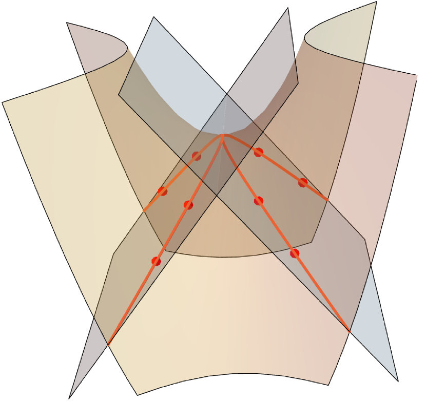
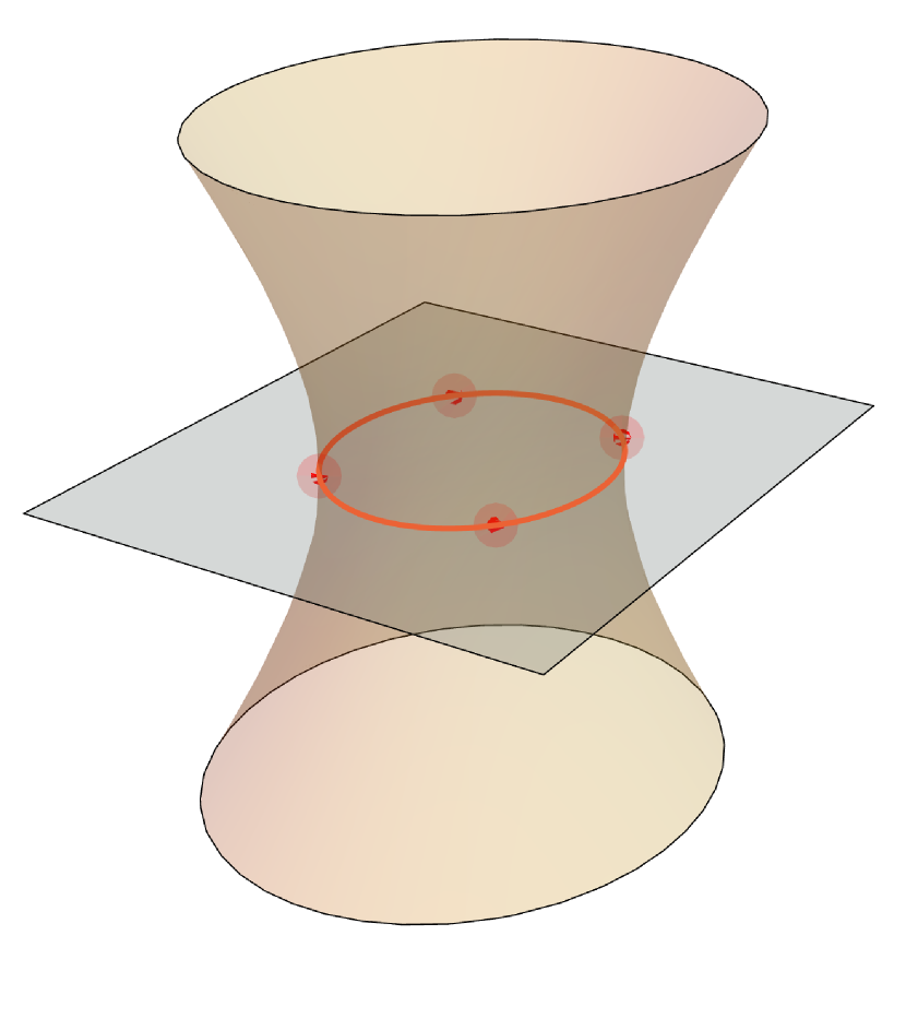
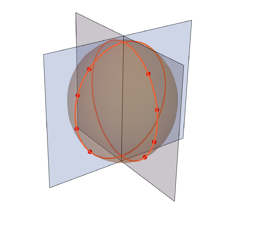
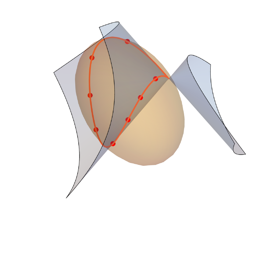
A pencil of quadrics in containing non-degenarate quadrics. Such pencils can be classified modulo projective transformations of , and they come in thirteen classes. The class of the pencil can be identified by the type of its base curve . This is a spatial curve of degree 4, whose type can vary from a generic one (irreducible smooth curve for a pencil of type (i)), through irreducible curves with a node (type (ii)) or with a cusp (type (iii)), to various types of reducible curves (from two non-coplanar conics intersecting at two points, type (iv), to a pair of intersecting double lines, type (xiii)).
-
•
The second pencil of quadrics having one quadric in common with , say . The base curves of both pencils intersect at eight points , .
-
•
Given two pencils of quadrics, one can define a three-dimensional analog of a QRT map , where the 3D QRT involutions , act along two families of generators of , see [1]. Each involution puts into correspondence two intersection points of a generator with the quadric . By definition, such an involution, and therefore the 3D QRT map , leaves each quadric of two pencils invariant, and thus possesses two rational integrals of motion and .
-
•
A Painlevé deformation map is the device which allows us to travel across the pencil . More precisely, such a map on preserves the pencil, but not fiber-wise. Rather, it sends each quadric to a different quadric . Moreover, preserves the base curve of the pencil . In the cases considered in [2], the base curve is reducible and contains straight lines. In these cases, does not necessarily fix these straight lines point-wise. In the cases considered in the present paper, fixes the base curve pointwise (in particular, it fixes all eight points ).
-
•
A 3D Painlevé map is obtained by composition , provided it possesses the singularity confinement property. It is to be stressed that the pencil continues to play a fundamental role in the dynamics of : the maps , preserve the pencil and map each quadric to . We do not have a straightforward description of the dynamical role of the pencil , but anticipate its relation to the isomonodromic description of the discrete Painlevé equations.
One can say that in our approach the role of a family of generalized Halphen surfaces is played by the quadrics of the pencil with eight distinguished points on the base curve of the pencil. The base curve itself plays the role of the unique anti-canonical divisor. Let us stress several features of our construction which are in a sharp contrast to the Sakai scheme.
-
•
Neither the exceptional divisor nor the eight distinguished points evolve under the map . Their discrete time evolution is apparent and is due to their representation in the so-called pencil-adapted coordinates. These are coordinates establishing an isomorphism between each quadric of the pencil and . The pencil-adapted coordinates of a point on the base curve do depend on , so traversing the pencil under induces an apparent discrete time evolution of the base curve and of the eight distinguished points.
-
•
The shift parameter of discrete Painlevé equations (or its exponent for the -difference equations among them) is not an intrinsic characteristic of the configuration of eight distinguished points, but is a free parameter of the construction.
One can say that our approach is a realization of the old-style idea of discrete Painlevé equations being non-autonomous versions (or modifications) of the QRT maps. This idea was instrumental in the discovery and early classification attempts of discrete Painlevé equations, summarized in [8]. A more geometric version of this procedure was proposed in the framework of the Sakai’s scheme by Carstea, Dzhamay and Takenawa [5]. In their scheme, the de-autonomization of a given QRT map depends on the choice of one biquadratic curve of the pencil. In our approach, the choice of the base curve and eight distinguished point on it determines uniquely all the ingredients of the construction, starting with the two pencils of quadrics.
The structure of the paper is as follows. In Section 2, we describe the construction scheme of discrete Painlevé equations applicable to the present case and stress its distinctions from the previous paper [2]. The main distinction is that here we consider the pencils whose characteristic polynomial is not a complete square. As a consequence, the 3D QRT involutions , and the 3D QRT map are no more birational maps of . Rather, these maps become birational maps on , a branched double covering of , whose ramification locus is the union of the singular quadrics , where are the branch points of the Riemann surface of .
In Section 3, we formulate a general recipe for the construction of the Painlevé deformation map , responsible to the evolution across the pencil of quadrics . While in the first part [2] we had , where is a Möbius automorphism fixing the set , in the present paper the natural definition becomes , where is the holomorphic uniformization map for the Riemann surface , and is the translation on the universal cover . The recipe turns out to be applicable to all types of the pencil except for the generic type (i). The latter leads to the elliptic Painlevé equation, which will be treated in a separate publication.
In Section 4, we show that the so constructed ensures the fundamental singularity confinement property for our 3D Painlevé maps.
There follow five Sections 5–9 containing a detailed elaboration of our scheme for all relevant types of the pencils except for the type (i). We recover, within our novel framework, all discrete Painlevé equations except for the elliptic one, which is left for a separate publication.